Analyzing events with a duration in DAX

UPDATE 2020-11-10: You can find more complete detailed and optimized examples for this calculation in the DAX Patterns: Events in progress article+video on daxpatterns.com.

Whenever we speak about orders, we think at sale orders. In a more generic way, an order is a request that you make and that requires some work to be completed, like an order to some machinery that builds stuff, an order to a software developer to build a website, or the request to accomplish any kind of work. All these types of orders have a start date, an end date and, many times, you are interested in understanding and aggregating what is happening between the two dates. The canonical way of modeling similar scenarios is to use two dates or time columns associated to the same entity or the same event. You cannot associate such an element to a single point in time, because the effects span over a period of time. This is one of the many examples which are covered in the new book about data modeling for Excel and Power BI.

When it comes to build data models to handle events, you always need to carefully balance usability, clarity and performance. In fact, events are facts that, instead of existing in an instant in time (like sales, for example), have a duration. The duration might be a few hours, days or even years, it all depends on the business model you are working on. For an insurance company, for example, a contract with a customer might last for one year whereas for orders, they typically last for a few days, or even minutes. Nevertheless, the two models, although in different businesses, are just slight variations of the events data model.

The naïve interpretation of a data model for events is the following one, where we have customers, date and orders. Each order has an order date and a ship date, and its duration lays between the two dates.

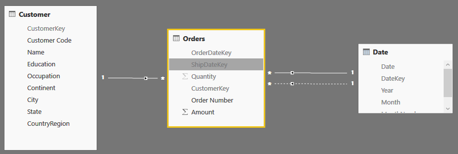
Since the fact table contains two dates, you can setup the two relationships between Orders and Date, one of which need to be kept inactive due to the well-known limitation of Tabular, which refuses to create ambiguous models.

The problem with this model is that you can easily browse the order amount sliced by order date, producing a report like the following one, but it is much harder to slice it by Ship Date, in case you want to see the amount of goods shipped instead of the amount ordered.

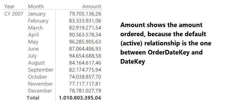
If you want to show a measure indicating the amount shipped, the way to go is not that of creating an additional date table. Instead, you should leverage the USERELATIONSHIP function and activate the inactive relationship for the duration of the calculation:

Amount Shipped := 
CALCULATE ( 
    SUM ( Orders[Amount] ), 
    USERELATIONSHIP ( Orders[ShipDateKey], 'Date'[DateKey] ) 
)

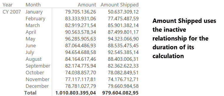
In this way, the Date dimension can slice by order and ship date, showing the correct numbers and still being the only date dimension in the model, as it should be:

So good for the appetizers, it is time to go for the main course. There are several interesting calculations you can perform with events; in this article we cover two of them:

1. Active orders, which is the number of orders that, in a given period, are active. An order is considered active between the order date and the ship date
2. Value of production, which is the amount produced every day. If it takes 10 days to produce an order of 5,000 USD, the daily production value of that order is 500 USD for each day.

Let us start from the active orders. On a single day, it is easy to determine whether an order is active or not, whereas at a more aggregate level you need do decide what to show. In fact, if you look at a whole month, many orders are opened and closed during the month. How do you want to account them? You have several choices. For example, you can show – at the month level – the number of orders that were active at the end of the month.
In this article, we go for a different calculation: we always show the average number of open orders in the selected period. At the day level, it will show the number of open orders. At a lower granularity, it shows a meaningful daily average of the open orders.

These are the formulas used in the next report:

Received Orders := COUNTROWS ( Orders )

Shipped Orders := 
CALCULATE ( 
    COUNTROWS( Orders ), 
    USERELATIONSHIP( Orders[ShipDateKey], 'Date'[DateKey] ) 
)

Active Orders =
AVERAGEX (
    VALUES ( 'Date'[DateKey] ),
    VAR CurrentDate = 'Date'[DateKey]
    VAR OrderedBeforeCurrentDate =
        FILTER ( 
            ALL ( Orders[OrderDateKey] ), 
            Orders[OrderDateKey] <= CurrentDate 
        )
    VAR ShippedAfterCurrentDate =
        FILTER ( 
            ALL ( Orders[ShipDateKey] ), 
            Orders[ShipDateKey] >= CurrentDate 
        )
    RETURN
        CALCULATE (
            COUNTROWS ( Orders ),
            OrderedBeforeCurrentDate,
            ShippedAfterCurrentDate,
            ALL ( 'Date' )
        )
)

It is worth to mention, in the code of Active Orders, the need of using ALL ( ‘Date’ ) to get rid of automatic filtering generated by the context transition produced by the CALCULATE function, which is called in the AVERAGEX iteration.
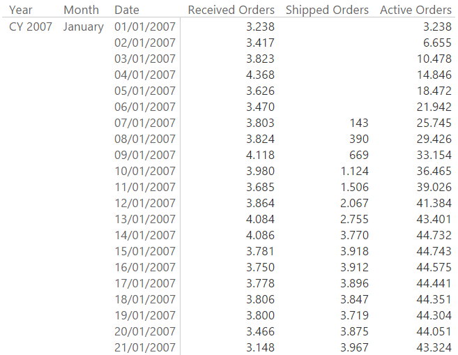
These three measures are already useful to produce interesting results:

Using SQL 2016 or Power BI, the formula performs nicely and further optimizations are not really needed. However, it is not a very fast measure and, worse, most of the time needed to compute the number of active orders is spent in the Formula Engine. Not only it results in sub-optimal performance, it also does not use the DAX cache the way it could.

Unfortunately, in order to speed up the calculation, you have to change the model, because the calculation relies on a logical relationship that is using less-than and greater-than conditions, whereas the VertiPaq engine can only handle equi-join conditions for physical relationships.

In this situation, a possible solution is that of materializing, in a calculated table, the number of orders open at a given date. The following code generates the OpenOrders table, which only contains the order number and the date, stating that – that day – the given order was open.

OpenOrders = 
SELECTCOLUMNS (
    GENERATE (
        Orders,
        FILTER (
            ALLNOBLANKROW ( 'Date' ),
            AND (
                'Date'[DateKey] >= Orders[OrderDateKey],
                'Date'[DateKey] <= Orders[ShipDateKey]
            )
        )
    ),
    "DateKey", 'Date'[DateKey],
    "Order Number", Orders[Order Number]
)

You can add the table to the data model and hide it, since it is a technical table needed only to compute the open orders:

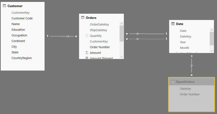
At this point, the number of active orders becomes much simpler to compute:

ActiveOrders := 
AVERAGEX ( 
    'Date', 
    CALCULATE ( COUNTROWS ( OpenOrders ) ) 
)

Obviously, the size of the OpenOrders table is much larger than the original one (in the demo file the Orders table has 1.6 million rows, whereas the OpenOrders table contains 18 million rows, which is 10 times larger). Nevertheless, because the calculation involves only the Storage Engine, it performs much better than the previous calculation on the smaller table, both with warm and cold cache. Because the size of the OpenOrders table strongly depends on the number of days for which an order is open, your mileage may vary a lot, depending on the kind of business you are modeling.

Moreover, with the physical table for open orders, computing the total number of orders that were open – at any time – during a month or a quarter becomes much simpler than with the previous model. Basically, by creating the calculated table, we moved at process time the task of computing whether an order is open or closed. By doing this, we left at query time only the task of counting the open orders, which is much faster.

Before taking for granted that this is the best solution, please note that by precomputing the table, we are fixing the granularity at the order level. In our example, it is likely that an order relates to a single customer, so that you can revisit the model, relate customers to orders and fix the issue. Nevertheless, on a more complex model, this operation might not be so easy. In such a case, you need to either work with the granularity of the snapshot table, increasing it, or at least protect the formulas so that you do not show numbers that – given the model – cannot be computed.

Now, let us move to the daily value of production. In this case, you need to find how many orders were open at a given point in time, and you also need to compute, for each order, the value it produced in that given day. If you have worked on an order for x days, its daily value can be obtained by dividing the total amount by x. On the original model, the pattern is similar to the previous one but, this time, the code is a bit harder to author.

The most intuitive way of computing the value in a measure might be the following one, which is easy to understand and use, if you don’t worry at all about performance. In fact, it is a slight variation of our first trial for open orders, but even on a small 1.6 million rows table, the time it takes to compute the result is huge: more than one minute for a simple report, all of this time is spent in Formula Engine.

Production Value :=
AVERAGEX (
    VALUES ( 'Date'[DateKey] ),
    VAR CurrentDate = 'Date'[DateKey]
    VAR OrderedBeforeCurrentDate =
        FILTER ( 
            ALL ( Orders[OrderDateKey] ), 
            Orders[OrderDateKey] <= CurrentDate 
        )
    VAR ShippedAfterCurrentDate =
        FILTER ( 
            ALL ( Orders[ShipDateKey] ), 
            Orders[ShipDateKey] >= CurrentDate 
        )
    RETURN
        CALCULATE (
            SUMX (
                Orders,
                DIVIDE (
                    Orders[Amount],
                    LOOKUPVALUE ( 
                        'Date'[Date], 
                        'Date'[DateKey], 
                        Orders[ShipDateKey] 
                    )
                        - RELATED ( 'Date'[Date] )
                )
            ),
            OrderedBeforeCurrentDate,
            ShippedAfterCurrentDate,
            ALL ( 'Date' )
        )
)

Of course, by materializing the daily production value in a calculated column, you can save some time because the innermost DIVIDE would become a calculated column. Yet, you see that when calculations start to grow in complexity, the formula becomes slower and slower. Beside, Formula Engine is still the main CPU eater, and this is no good at all.

Luckily, if you followed the article so far, you might notice that the same optimization we used earlier is going to be extremely efficient here. In fact, you can precompute the daily production value of an order and store it in the same table where you previously stored the open orders. Again, you perform the heavy calculation earlier (by computing the daily production value of an order), and you execute at query time only sum of these pre-calculated values.

The code for Open Orders requires more lines of DAX code, because of the calculation of the daily production rate inside the query, in order to materialize its result in the calculated table.

OpenOrders = 
SELECTCOLUMNS (
    GENERATE (
        ADDCOLUMNS (
            Orders,
            "DailyProductionValue", DIVIDE (
                Orders[Amount],
                LOOKUPVALUE ( 
                    'Date'[Date], 
                    'Date'[DateKey], 
                    Orders[ShipDateKey] 
                )
                    - RELATED ( 'Date'[Date] )
            )
        ),
        FILTER (
            ALLNOBLANKROW ( 'Date' ),
            AND (
                'Date'[DateKey] >= Orders[OrderDateKey],
                'Date'[DateKey] <= Orders[ShipDateKey]
            )
        )
    ),
    "DateKey", 'Date'[DateKey],
    "Order Number", Orders[Order Number],
    "DailyProductionValue", [DailyProductionValue]
)

On the other hand, the formula to compute the production value becomes a simple SUM:

Production Value = SUM ( OpenOrders[DailyProductionValue] )

With these measures in place, the following report, showing received, shipped and active orders along with the production value is rendered in a few milliseconds, as you can easily try by yourself by downloading the sample file for Power BI Desktop. Please note that, in order to reduce its size, we removed the solution from the demo file, you will need some copy & paste to make it a working one.

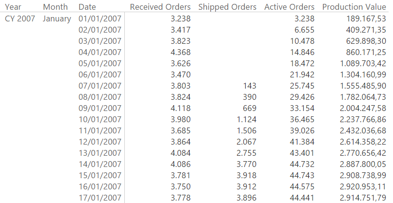
It is worth to note – again – that the granularity might be an issue. In fact, if you need to re-allocate the production value by other dimensions and not only by date, then you will need to take many complex decisions in order to split the production value by those dimensions. Nevertheless, these are problems of the specific business, the goal of the article is to show a simple example to approach the issue. You have to customize the model for your specific requirements.

As you have seen in this article, data modeling plays a very important role in the definition of a business solution, even if it is a simple Power BI file you want to use to track the productivity of your team. Using the correct model, the formulas tend to be much simpler and faster. If you do not pay attention at the model using the naïve solutions, you end up writing slower and more complex DAX expressions.