 Marco Russo & Alberto Ferrari
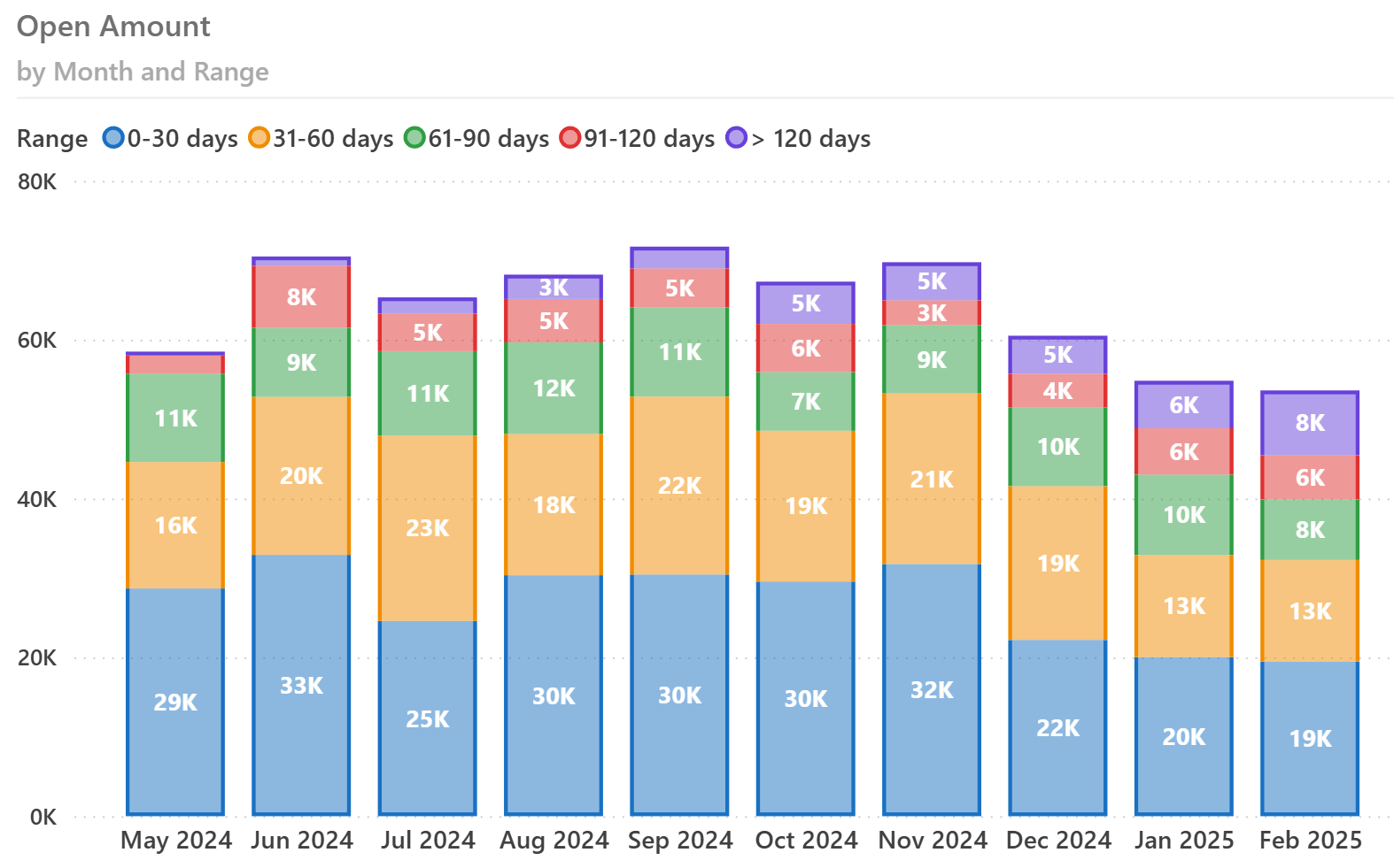
The Accounts Receivable (AR) Aging report helps companies track overdue receivables and better manage their cash flow. It is a common requirement from the finance department that often represents a challenge for Power BI reports, especially when you want to show the trend over time. Here is a typical visualization for the Open Amount at the end of each month, colored by the age range of the Accounts Receivable.
This article demonstrates how to implement a flexible and scalable AR Aging solution in Power BI and how to simplify a business problem using standard modeling patterns.
The source data model is almost never good
While the AR Aging report is pretty standard, the source data can have a variety of formats that typically do not fit the requirements:
- One Big Table: Implementing an interactive Power BI report is challenging with a flat file or a unified table with no relationships.
- OLTP Systems: Transaction-based relational databases optimized for data entry, not analytics. Usually, these data sources have a large number of tables and relationships, requiring expensive calculations to generate aggregated results.
- Data Marts / Warehouses: Data structures optimized for reporting but sometimes lacking the detail or flexibility required to reflect nuances in AR Aging.
These common data models rarely provide an ideal structure for AR Aging reports. They often include:
- Complex joins or missing relationships make tracking invoice status or partial payments difficult.
- Limited ability to handle partial credits, deferred payments, or adjustments that occur over time.
- Challenges in aligning specific business rules (e.g., different aging buckets, currency conversions, or discount terms) with the raw transactional data.
Hence, importing the data as-is usually requires complex DAX measures to provide the necessary result, and creating five identical reports for five different customers typically requires five completely different models and measures. To avoid this, we first transform the data into a model that better suits the requirements. We may use well-known modeling patterns to simplify or at least standardize the process once we reach a specific data format that better supports it.
Model the problem
Let us introduce a data source that provides the information in three tables: Invoices, Payments Due, and Payments. Each table has the granularity of the entity represented. Data in different tables is linked through the Invoice number, even though the customer information is also part of each table.
The Invoice table has one row for each invoice, and the row shows the details down to the payment terms.
| Customer | Invoice | Date | Amount | Terms |
|---|---|---|---|---|
| Litware | INV-001 | 9/15/2024 | 10,000 | 30 |
| Litware | INV-002 | 9/15/2024 | 16,000 | 60/90 |
| Contoso | INV-003 | 9/15/2024 | 3,000 | 15 |
The Payments Due table could be inferred from the Invoice table. However, we assume it is already available in this form, so we do not make any assumptions about existing payment terms. This way, we can manage any exception or manual payment term assigned in arbitrary ways.
| Customer | Invoice | Due Date | Amount Due |
|---|---|---|---|
| Contoso | INV-003 | 9/30/2024 | 3,000 |
| Litware | INV-001 | 10/15/2024 | 10,000 |
| Litware | INV-002 | 11/15/2024 | 8,000 |
| Litware | INV-002 | 12/15/2024 | 8,000 |
The Payments table contains one row for each payment as it is assigned to an invoice. If a single payment references multiple invoices, the amount must be split into the corresponding invoices in this table (see the payment on 12/30/2024, which allocates $3,000 to INV-001 and $12,000 to INV-002). This way, we can incorporate into our model the situations where a customer intentionally suspended payment for an invoice but continued the payments for the following.
| Customer | Invoice | Payment Date | Payment Amount |
|---|---|---|---|
| Contoso | INV-003 | 9/30/2024 | 3,000 |
| Litware | INV-001 | 10/30/2024 | 7,000 |
| Litware | INV-001 | 12/30/2024 | 3,000 |
| Litware | INV-002 | 12/30/2024 | 12,000 |
| Litware | INV-002 | 1/30/2025 | 2,000 |
Suppose the available data does not allow this because you do not have the invoice reference in the payment data. When you cannot allocate the payments to the invoice (like when you only have Customer, Payment Date, and Payment Amount), you can consider allocating the payment to the invoices in a way we will be showing later, that allocates payments on due dates.
Can you create a DAX query based on these three tables? Certainly, yes. However, that solution would face the complexity of reconciling payments received with due dates at query time. We want to avoid that scenario because the code to write is more complex, error-prone, challenging to reuse in different models, and potentially slow.
Ideally, we want a model with a single “fact” table for the Account Receivable data, with a granularity corresponding to the intersection of payments due and payments so that every row is part of the payment allocated to a due date for one invoice. This is the AR Detail table we want to use in our model: you should notice that INV-002 has four rows, even though that invoice has two rows in Payments Due and two rows in Payments.
| Customer | Document | Amount Due | Due Date | Amount Paid | Payment Date |
|---|---|---|---|---|---|
| Contoso | INV-003 | 3,000 | 9/30/2024 | 3,000 | 9/30/2024 |
| Litware | INV-001 | 7,000 | 10/15/2024 | 7,000 | 10/30/2024 |
| Litware | INV-001 | 3,000 | 10/15/2024 | 3,000 | 12/30/2024 |
| Litware | INV-002 | 8,000 | 11/15/2024 | 8,000 | 12/30/2024 |
| Litware | INV-002 | 4,000 | 12/15/2024 | 4,000 | 12/30/2024 |
| Litware | INV-002 | 2,000 | 12/15/2024 | 2,000 | 1/30/2025 |
| Litware | INV-002 | 2,000 | 12/15/2024 |
You can create the AR Detail table starting from the source data. However, this transformation is particularly challenging and time-consuming from a development perspective. Therefore, we prefer to add an intermediate step starting from a standard, normalized format of the events we want to analyze. The goal is to reuse the complex transformation from the normalized format to the AR Detail table in every new model, and leave to the customization step only the easier task of populating the normalized Movements table we describe in the following section.
Normalizing movements
As we have seen, the source data often includes separate tables for invoices and payments. Each table might have different columns and relationships. To simplify the solution, we create a normalized Movements table that unifies these various transaction types into one standard structure.
| Customer | Document | Type | Amount | Date |
|---|---|---|---|---|
| Litware | INV-001 | Invoice | 10,000 | 9/15/2024 |
| Litware | INV-001 | Payment Due | 10,000 | 10/15/2024 |
| Litware | INV-001 | Payment | 7,000 | 10/30/2024 |
| Litware | INV-001 | Payment | 3,000 | 12/30/2024 |
| Litware | INV-002 | Invoice | 16,000 | 9/15/2024 |
| Litware | INV-002 | Payment Due | 8,000 | 11/15/2024 |
| Litware | INV-002 | Payment Due | 8,000 | 12/15/2024 |
| Litware | INV-002 | Payment | 12,000 | 12/30/2024 |
| Litware | INV-002 | Payment | 2,000 | 1/30/2025 |
| Contoso | INV-003 | Invoice | 3,000 | 9/15/2024 |
| Contoso | INV-003 | Payment Due | 3,000 | 9/30/2024 |
| Contoso | INV-003 | Payment | 3,000 | 9/30/2024 |
This article does not cover the transformation to obtain the Movements table. In the sample files, you will find a solution (AR Aging – sample) that has the Movements table loaded with the content described in the table above, plus additional documents. A second solution (AR Aging – volume) creates a larger number of rows in Movements depending on the definition of the hidden Parameters table. You can use the large volume to test the effectiveness of the optimizations we will describe later in the article.
The Movements table enables the analysis of invoices, payments due, and payments grouped by date using a single date table. Indeed, Movements is a fact table in a regular star schema.
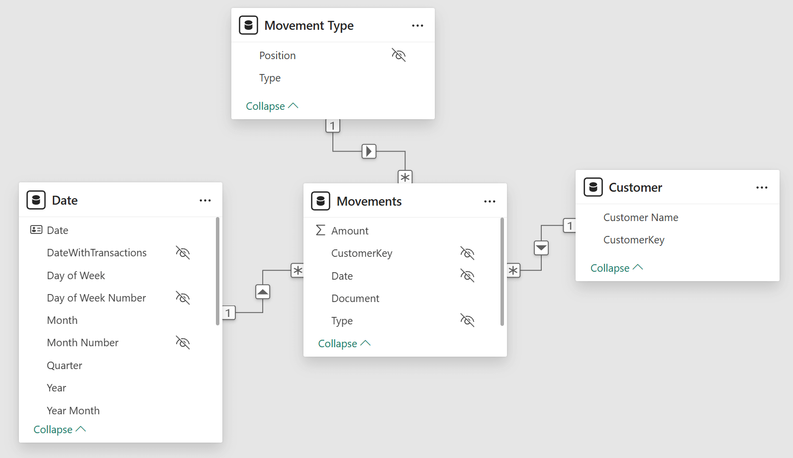
You can easily create reports like the following without writing any DAX measure.
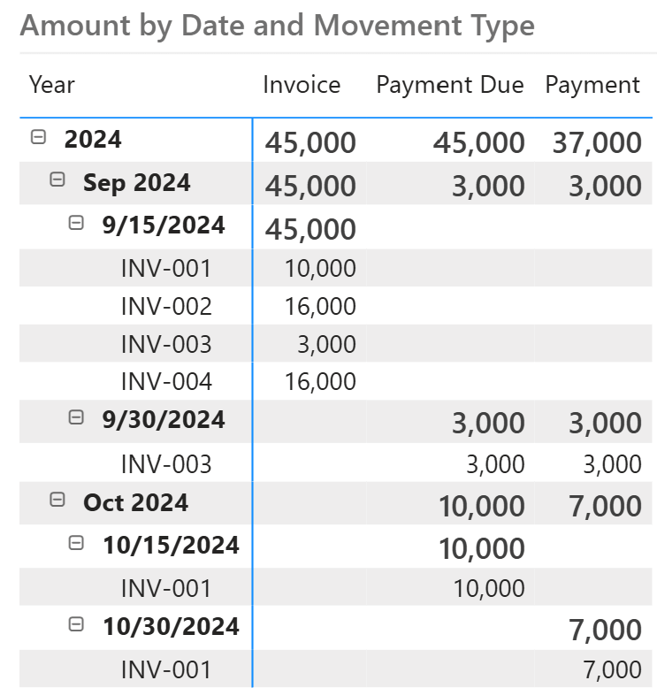
However, the AR Aging report requires some additional effort. The good news is that if you can adapt your model to the Movements table structure we just described, you can easily reuse the model and measures described in the remaining part of the article to get a working AR Aging solution.
Implementing AR Detail from normalized movements
How do you obtain the AR Detail table we described at the beginning of the article, starting from the Movements table we just analyzed? Well, you can use the data transformation tool you are more comfortable with. For example, you could implement the transformation in SQL or in Power Query. A complex solution can populate the AR Detail incrementally, reducing the processing time for every refresh. It is important to highlight that a transformation is necessary because it is very unlikely that your data source already has the precise structure and granularity we want for AR Detail. Therefore, this kind of reporting does not work well in a real-time environment – we have to take into account the latency required by the transformation for AR Detail, wherever it may happen.
If you have a relatively small amount of data, you may consider a calculated table in DAX, which is what we describe in this article. The advantage of this approach is that the AR Detail table is guaranteed to be synchronized with the other tables in the model: we expect this to be an additional feature of an existing semantic model rather than a separate semantic model created just for this purpose. To quantify a “small amount of data”, we can assume that any number below 1 million payments due should be acceptable. In contrast, if you have more than 10 million payments due, you may want to consider alternative approaches allowing an incremental update of that table.
We do not describe the DAX implementation of the AR Detail calculated table in detail. Indeed, we did not look for the most efficient implementation; we tried to split the calculation into multiple steps using variables that you can inspect to understand how this code works.
AR Detail =

VAR AmountsDueRaw =
    CALCULATETABLE (
        ADDCOLUMNS (
            SUMMARIZE (
                Movements,
                Movements[CustomerKey],
                Movements[Document],
                Movements[Date]
            ),
            "AmountDue", CALCULATE ( SUM ( Movements[Amount] ) )
        ),
        Movements[Type] = "Payment Due"
    )

VAR AmountsDue =
    SELECTCOLUMNS (
        AmountsDueRaw,
        Movements[CustomerKey],
        Movements[Document],
        Movements[Date],
        "CumulDue",
            SUMX (
                WINDOW (
                    0, ABS,
                    0, REL,
                    AmountsDueRaw,
                    ORDERBY ( [Date], ASC ),
                    PARTITIONBY ( [Document], [CustomerKey] ),
                    MATCHBY ( [Date] )
                ),
                [AmountDue]
            ),
        "PrevCumulDue",
            SUMX (
                WINDOW (
                    0, ABS,
                    -1, REL,
                    AmountsDueRaw,
                    ORDERBY ( [Date], ASC ),
                    PARTITIONBY ( [Document], [CustomerKey] ),
                    MATCHBY ( [Date] )
                ),
                [AmountDue]
            )
    )

VAR AmountsPaidRaw =
    CALCULATETABLE (
        ADDCOLUMNS (
            SUMMARIZE (
                Movements,
                Movements[CustomerKey],
                Movements[Document],
                Movements[Date]
            ),
            "AmountPaid", CALCULATE ( SUM ( Movements[Amount] ) )
        ),
        Movements[Type] = "Payment"
    )

VAR AmountsPaid =
    SELECTCOLUMNS (
        AmountsPaidRaw,
        Movements[CustomerKey],
        Movements[Document],
        "PaidDate", Movements[Date],
        "CumulPaid",
            SUMX (
                WINDOW (
                    0, ABS,
                    0, REL,
                    AmountsPaidRaw,
                    ORDERBY ( [Date], ASC ),
                    PARTITIONBY ( [Document], [CustomerKey] ),
                    MATCHBY ( [Date] )
                ),
                [AmountPaid]
            ),
        "PrevCumulPaid",
            SUMX (
                WINDOW (
                    0, ABS,
                    -1, REL,
                    AmountsPaidRaw,
                    ORDERBY ( [Date], ASC ),
                    PARTITIONBY ( [Document], [CustomerKey] ),
                    MATCHBY ( [Date] )
                ),
                [AmountPaid]
            )
    )

VAR DetailPayments =
    GENERATEALL (
        NATURALLEFTOUTERJOIN ( AmountsDue, AmountsPaid ),
        VAR curDueMax =
            MIN ( [CumulDue], [CumulPaid] ) -- LEAST
        VAR curDueMin =
            MAX ( [PrevCumulDue], [PrevCumulPaid] ) -- GREATEST
        VAR AmountPaid =
            IF ( curDueMax - curDueMin > 0, curDueMax - curDueMin, 0 )
        RETURN ROW (
            "curDueMax", curDueMax,
            "curDueMin", curDueMin,
            "Payment Amount", AmountPaid
        )

    )

VAR LeftoverStep1 =
    GROUPBY (
        DetailPayments,
        Movements[CustomerKey],
        Movements[Document],
        Movements[Date],
        "AmountPaid", SUMX ( CURRENTGROUP (), [Payment Amount] )
    )

VAR LeftoverStep2 =
    ADDCOLUMNS (
        NATURALLEFTOUTERJOIN(
            AmountsDueRaw,
            LeftoverStep1
        ),
        "Leftover", [AmountDue] - [AmountPaid]
    )
VAR LeftoverByDueDate =
    SELECTCOLUMNS (
        LeftoverStep2,
        Movements[CustomerKey],
        Movements[Document],
        "Due Date", CONVERT ( Movements[Date], DATETIME ),
        "Amount Due", [LeftOver],
        "Payment Date", CONVERT ( BLANK(), DATETIME ),
        "Payment Amount", CONVERT ( BLANK(), CURRENCY )
    )

VAR DetailPaymentsByDueDate =
    SELECTCOLUMNS (
        FILTER ( DetailPayments, [Payment Amount] > 0 ),
        Movements[CustomerKey],
        Movements[Document],
        "Due Date", Movements[Date],
        "Amount Due", [Payment Amount],
        "Payment Date", [PaidDate],
        "Payment Amount", [Payment Amount]
    )

VAR ArDetailRaw =
    UNION (
        DetailPaymentsByDueDate,
        FILTER ( LeftoverByDueDate, [Amount Due] <> 0 )
    )

VAR AR_Detail =
    SELECTCOLUMNS (
        ArDetailRaw,
        "Document", Movements[Document],
        "CustomerKey", Movements[CustomerKey],
        "Invoice Date",
            LOOKUPVALUE (
                Movements[Date],
                Movements[Document], Movements[Document],
                Movements[CustomerKey], Movements[CustomerKey],
                Movements[Type], "Invoice"
            ),
        "Amount Due", [Amount Due],
        "Due Date", [Due Date],
        "Amount Paid", [Payment Amount],
        "Payment Date", [Payment Date]
    )

RETURN AR_Detail
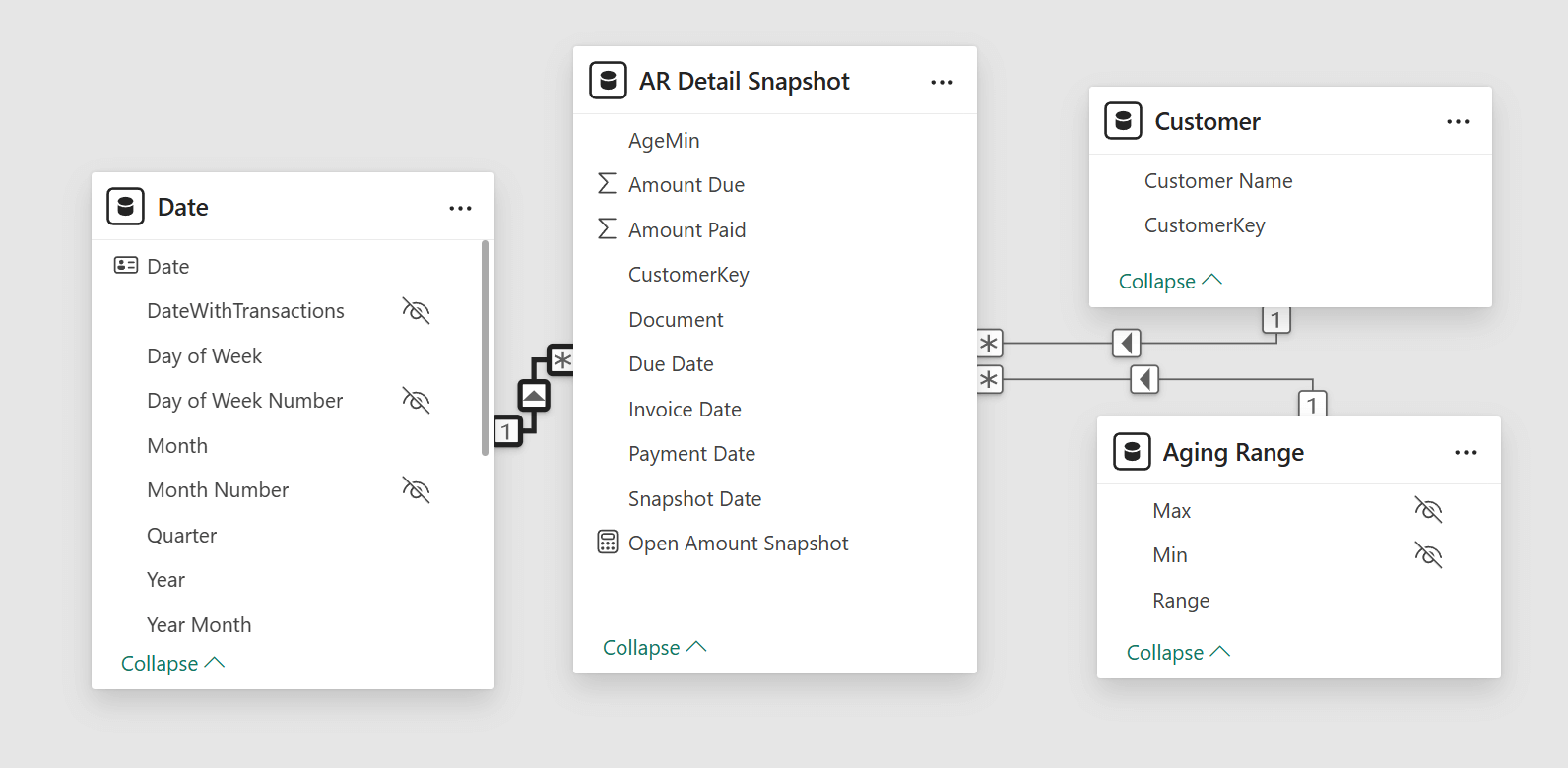
The AR Detail table is a fact table in a star schema that we connect to Customer and Date. The Aging Range table defines the aging buckets for the report, which we will describe later in the article.
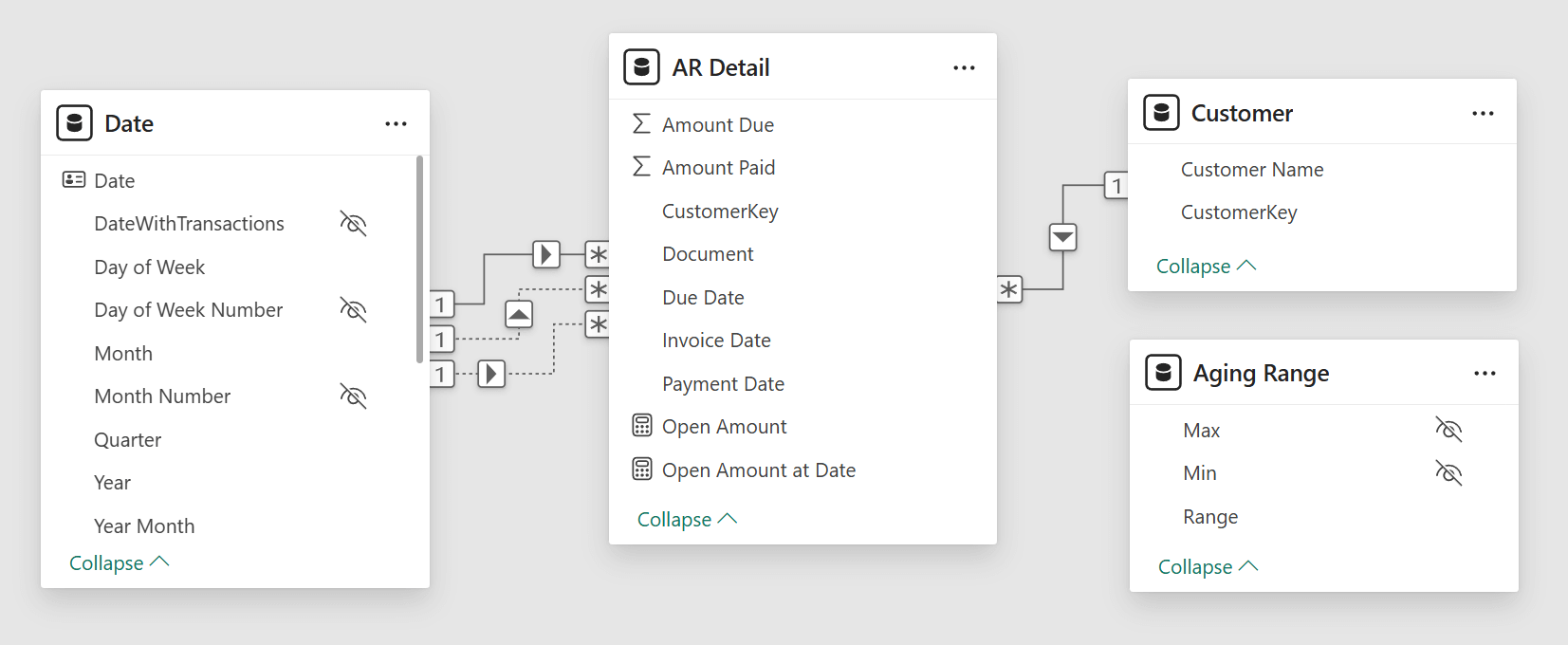
In this case, we see multiple relationships with Date, because each row in AR Details has three dates: Invoice Date, Due Date, and Payment Date. The last two are the ones we use to measure the age of each row in AR Detail, as we describe in the next section.
Applying DAX patterns
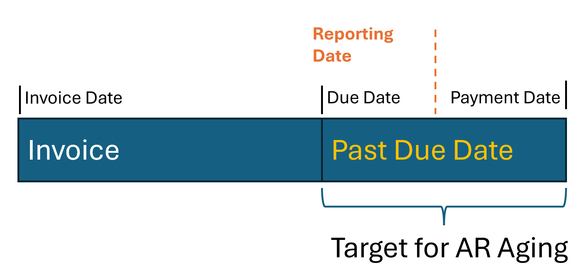
We have two requirements for creating the AR Aging report. First, we must obtain the amount “due” at a given date. We call this the “Open Amount”. Every row in AR Detail can project the same amount due for any reporting date between the Due Date and the Payment Date.
We have to write some DAX code for this but do not have to reinvent the wheel. This problem is just one case of the generic Events in progress pattern. You can follow the link to read how the calculation works. This is the code adapted to AR Detail to calculate the Open Amount on the reporting date:
Open Amount at Date =
VAR MaxDate =
    MAX ( 'Date'[Date] )
VAR Result =
    CALCULATE (
        SUM ( 'AR Detail'[Amount Due] ),
        'AR Detail'[Due Date] <= MaxDate,
        'AR Detail'[Payment Date] > MaxDate || ISBLANK ( 'AR Detail'[Payment Date] ),
        REMOVEFILTERS ( 'Date' )
    )
RETURN
    Result
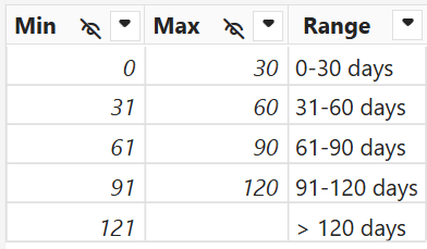
We are only halfway there to get the AR Aging report. Indeed, we must compute the age of each amount and allocate that in the corresponding range, using the Range column from the Aging Range table in our report. This is the content of Aging Range, which we might import from an external source (like a SharePoint table) to give users maximum flexibility.
Once again, we use another existing pattern, the Dynamic segmentation. For performance reasons, we merge the calculation into a single Open Amount measure to get a more efficient execution by reducing the number of context transitions:
Open Amount =
VAR MaxDate =
    MAX ( 'Date'[Date] )
VAR Result =
    CALCULATE (
        VAR _AgeDetail =
            ADDCOLUMNS (
                'AR Detail',
                "@AgeMin",
                    VAR _Age =
                        CONVERT ( MaxDate - 'AR Detail'[Due Date], INTEGER )
                    VAR _AgeMin =
                        SELECTCOLUMNS (
                            FILTER (
                                ALLNOBLANKROW ( 'Aging Range' ),
                                'Aging Range'[Min] <= _age
                                    && (
                                        'Aging Range'[Max] >= _age
                                            || ISBLANK ( 'Aging Range'[Max] )
                                    )
                            ),
                            'Aging Range'[Min]
                        )
                    RETURN
                        _AgeMin
            )
        VAR Result =
            SUMX (
                FILTER (
                    _AgeDetail,
                    NOT ISBLANK ( [@AgeMin] )
                        && [@AgeMin] IN VALUES ( 'Aging Range'[Min] )
                ),
                'AR Detail'[Amount Due]
            )
        RETURN
            Result,
        'AR Detail'[Due Date] <= MaxDate,
        'AR Detail'[Payment Date] > MaxDate || ISBLANK ( 'AR Detail'[Payment Date] ),
        REMOVEFILTERS ( 'Date' )
    )
RETURN
    Result
You can test the correctness of the calculation by playing with the data in the “AR Aging – sample.pbix” file included in the downloadable ZIP file: modify the content of the Movements calculated table to test corner cases you might want to consider, and validate the calculation before using the model for your specific scenario.
When it comes to performance, you should use the “AR Aging – volume.pbix” file. Increase the values assigned to _Customers and _Invoices variables in the Parameters table. While we provide the sample file with 1,000 invoices, if you use 1,000,000 as the number of invoices, you might wait up to one minute to refresh the calculated tables. At that point, the chart we had shown at the beginning of the article could require many seconds to be refreshed. If your data volume reaches a similar size, you may want to consider an additional step to improve query performance. A specific section describes the optimization of the Events in progress pattern, which is based on a snapshot table you can create in many ways (as usual, external data preparation is better because it allows incremental updates). One of the ways is to use a DAX calculated table:
AR Detail Snapshot =
GENERATE (
    SELECTCOLUMNS (
        DISTINCT ( 'Date'[Year Month Number] ),
        "Snapshot Date", CALCULATE ( MAX ( 'Date'[Date] ) )
    ),
    VAR _MaxDate = [Snapshot Date]
    VAR _OpenAR =
        FILTER (
            ALLNOBLANKROW ( 'AR Detail' ),
            'AR Detail'[Due Date] <= _MaxDate
                && (
                    'AR Detail'[Payment Date] > _MaxDate
                        || ISBLANK ( 'AR Detail'[Payment Date] )
                )
        )
    VAR Result =
        ADDCOLUMNS (
            _OpenAR,
            "AgeMin",
                VAR _Age =
                    CONVERT ( _MaxDate - 'AR Detail'[Due Date], INTEGER )
                VAR _AgeMin =
                    SELECTCOLUMNS (
                        FILTER (
                            'Aging Range',
                            'Aging Range'[Min] <= _age
                                && (
                                    'Aging Range'[Max] >= _age
                                        || ISBLANK ( 'Aging Range'[Max] )
                                )
                        ),
                        'Aging Range'[Min]
                    )
                RETURN
                    _AgeMin
        )
    RETURN
        Result
)
The AR Detail Snapshot table can be connected to Aging Range, because it pre-calculates the age of the account receivable for every reporting date and stores the corresponding range into the AgeMin column.
The measure that uses the snapshot comes with a simpler implementation and a much faster execution:
Open Amount Snapshot =
IF (
    ISCROSSFILTERED ( 'Date' ),
    CALCULATE (
        SUM ( 'AR Detail Snapshot'[Amount Due] ),
         LASTDATE ( 'Date'[Date] )
    )
)
Conclusions
The Account Receivable (AR) Aging report is a common scenario that can be solved in a standardized way, starting from a well-known normalized data structure. We implemented an initial Movements table that standardizes the process of creating the model that better fits the analytics requirement for AR Aging: the AR Detail table must have the right granularity to simplify the dynamic calculation of the age of a row for any given reporting date. By leveraging well-known and optimized DAX patterns, we minimize the development effort and reduce the risk of implementation errors. We also take advantage of the performance optimization already available for such models.
While this article describes the solution of a specific scenario, consider using the same approach when facing a new business requirement: always try to reduce the problem to a list of smaller steps that make it possible to reuse generic patterns.