Bidirectional relationships and ambiguity in DAX

UPDATE: You can now filter a slicer by using a measure without using a bidirectional filter, read Filter slicers without using bidirectional filters in Power BI for more details.

A relationship can be set to be unidirectional – its default behavior – or bidirectional. In a unidirectional relationship the filter context is propagated from the one-side to the many-side, but not the other way around. In other words, in the following diagram a filter on Customer automatically filters Sales, whereas a filter on Sales propagates neither to Product nor to Customer or Date.

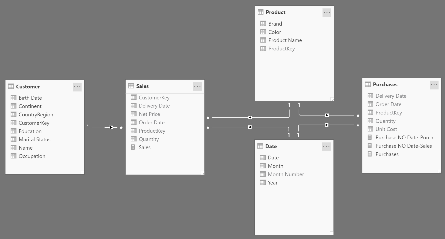
This behavior works well in most scenarios. Indeed, a report typically slices sales amount by customer or product attributes. It is quite uncommon to filter customers, or products, based on sales.

Therefore, why would one enable bidirectional filtering? The most common reason is to sync slicers.

Look at the following report where there are two slicers – one for the customer name and one for the product color, with a matrix providing sales details:

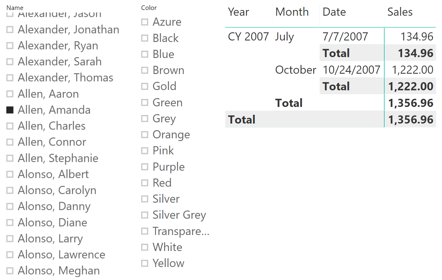
The report works well; it shows Amanda’s purchases. Nevertheless, the color slicer is not filtering the few colors purchased by Amanda. One can easily see which colors she bought by adding the color to the report, yet the slicer does not provide easy feedback to the user. The reason is that the filter on Customer reaches Sales. Therefore, it only filters the sales of the selected customer. But the filter does not automatically flow from Sales to Product, because the relationship between Product and Sales is set as a default unidirectional relationship.

There is an easy solution to the problem: set the relationship between Product and Sales as a bidirectional relationship. By doing that, the filter automatically propagates from Sales to Product, so that the slicer will only show the products (hence, the colors) of the selected customer. The result is quite nice:

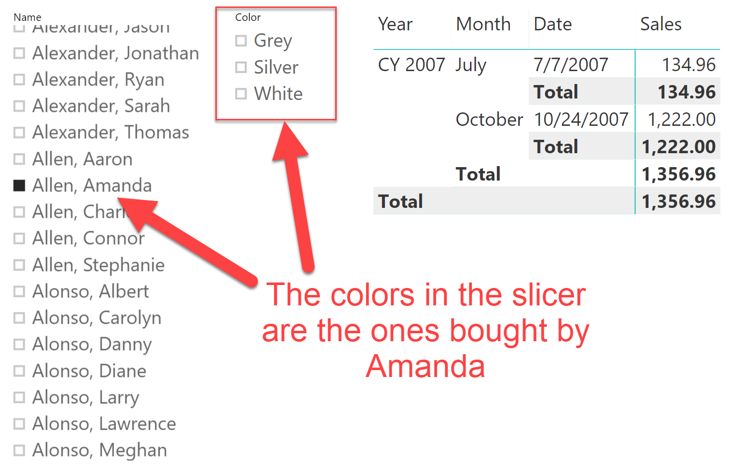
Several Power BI users rely on bidirectional filters for the purpose of syncing slicers. The model with unidirectional filters was simple and sound. The update of the relationship looked straightforward and convenient. Unfortunately, by enabling a simple bidirectional filter, the data model has now been transformed into a data monster, whose behavior is complex enough to be unpredictable. This is a strong statement, and the remainder of the article is devoted to that explanation.

First, let us look at the resulting model. It is not all that different from the original model. The only (tiny, not very noticeable) difference is the presence of the double arrow on the relationship between Sales and Product.

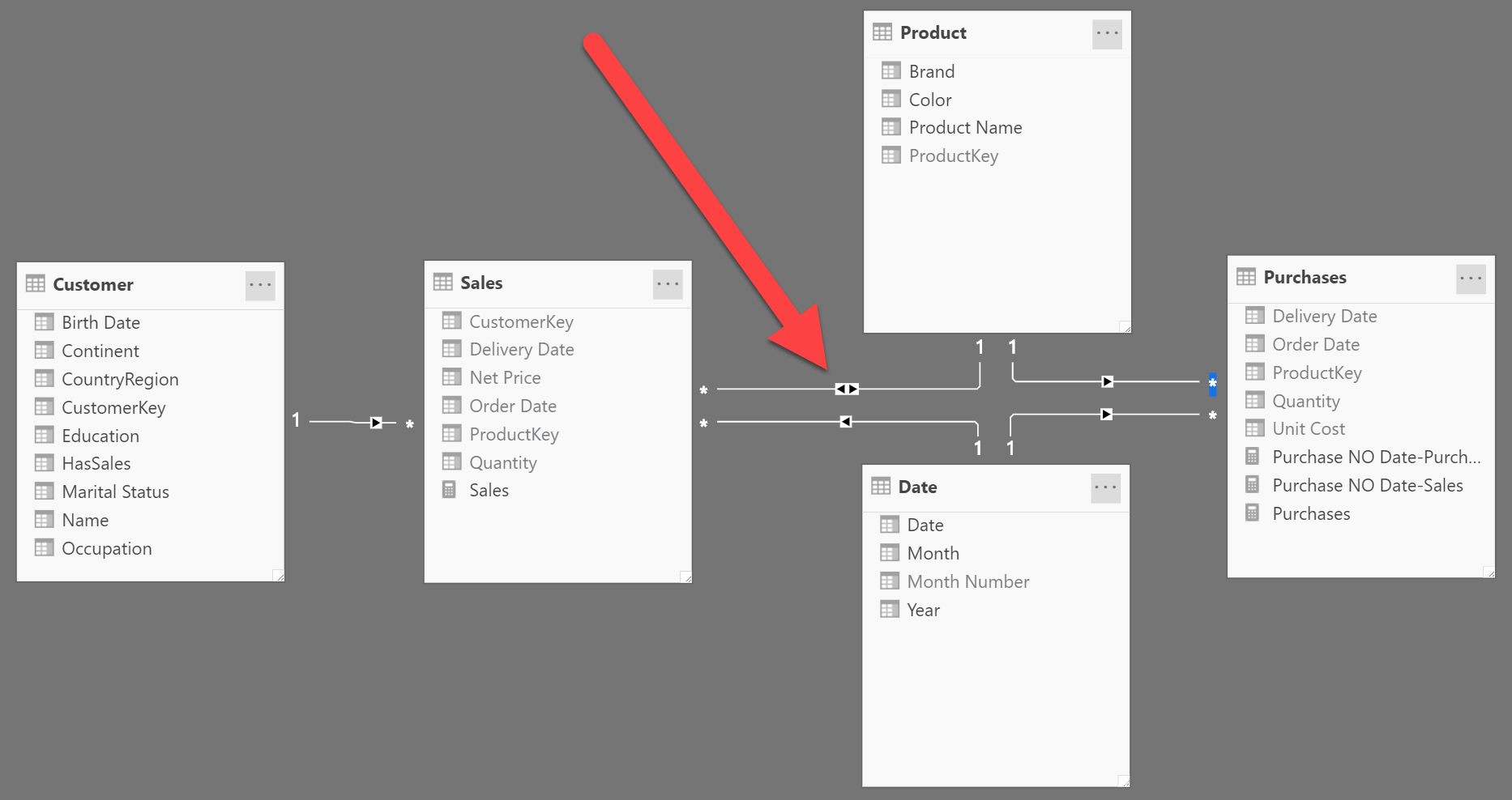
The presence of that bidirectional cross-filter is going to quickly create our worst nightmare, because it introduces ambiguity in the model. What is ambiguity? A model is ambiguous when there are multiple paths between tables. In an ambiguous model, the engine has multiple options when transferring a filter from one table to another. Therefore, it either finds a preferred way to transfer the filter, or it raises an error. In this scenario, no error was raised; therefore, either the model is not ambiguous (small spoiler: IT IS AMBIGUOUS), or the engine found a preferred way to transfer the filter.

Now, before moving on with the article, look at the model and check where the ambiguity is. You need to find two tables that are linked through different paths, following the arrows of the cross-filter. Hey, don’t cheat, stop reading and find these paths!

Ok, did you find them? Great! You discovered that starting from Date, you can reach Purchases in two different ways:

• From Date to Purchases: this is the direct relationship between the two tables, marked as (1) in the figure below.
• From Date to Sales, to Product, to Purchases: a much longer path, marked as (2) in the figure, which is perfectly legit.

You can see the two paths in the following figure:

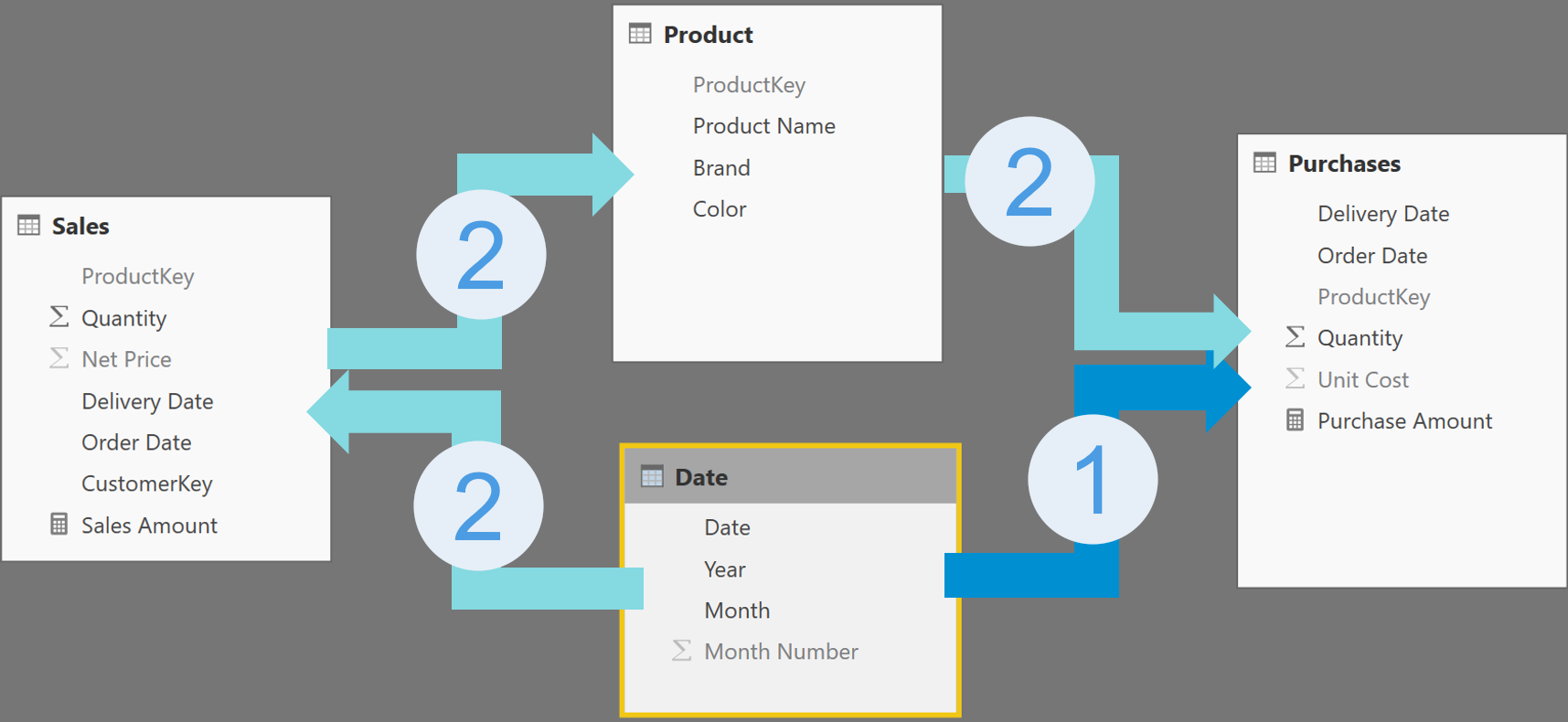
We created an ambiguous model, and yet the engine has not complained about it. The reason is that by analyzing the two paths, the engine has decided that one path is to be preferred against the other. The choice seems straightforward in this case: because one of the two relationships (number 1) is direct, it is the preferred path. Hence, when a filter needs to be moved from Date to Purchases, the engine uses the shortest path and avoids the longer one.

This scenario is artificially simple: there are two paths, one of which is clearly the best. It is utterly simple to create more complex scenarios where that choice is no longer obvious. Moreover, the algorithm used by the engine to choose the preferred path is not that trivial. Indeed, it does not just choose the shortest path. It chooses the shortest path where the first selecting relationship is closest to the filter. If this last sentence sounds confusing, that is by design. The algorithm is extremely complex to analyze and understand for a human. On average, the algorithm almost always picks the path that a human would have chosen, but in order to be a generic algorithm its description is much more complex. I will not be expanding on this any further.

Although one path is preferred over the other, there are still two possible paths to propagate the filter from Date to Purchases. In some scenarios, both paths can be travelled in a single expression, leading to ridiculous results. Let us elaborate on this.

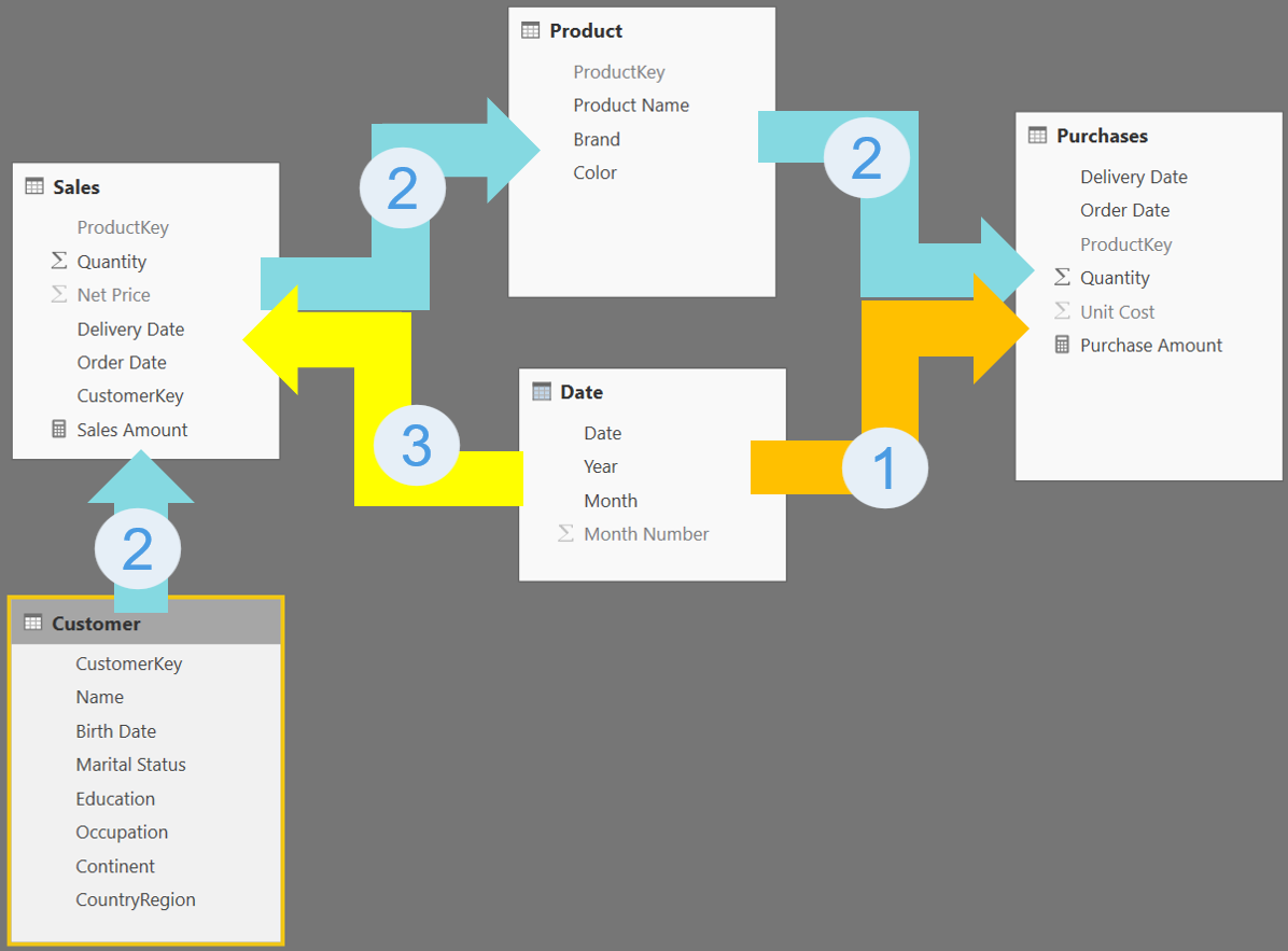
We know that a filter moves from Date to Purchases by following the most direct relationship. The following figure shows the full model, with colored and numbered paths.

Try to answer these simple questions about the model:

• Does Customer filter Purchases?
• Does Date filter Sales?
• If there is a filter on Date and a filter on Customer, do both filters apply to Sales? Moreover, if Sales is filtered by both Date and Customer, does this mean that Date filters Purchases through Sales?

The first two questions are simple. Customer filters Purchases by following path number 2. Date filters Sales following path number 3.

The third question is a bit more of a challenge. Sales is filtered by both Date and Customer. Date uses the yellow path (number 3), Customer uses the blue path (number 2), and both filter Sales. Then Sales reaches Purchases through the blue path (number 2). But at the same time, Date reaches Purchases through the orange path (number 1), and we already know that path number 1 is the preferred path. Therefore, which path does Date use to reach Purchases, when there is also a filter on Customer? I know, the scenario starts to be confusing. After all, we know the model is ambiguous. So the last question is just the logical conclusion of this reasoning: the more filters are present, the more ambiguity becomes an issue.

As I said, the algorithm that disambiguates the model is sophisticated. It finds its way through the maze of relationships even though the way it finds might not be the most intuitive one. The correct answer on this specific model is the following:

If Date and Customer are filtered, both filters are used against Sales. Then Sales filters Product which in turn filters Purchases. The yellow (3) relationship between Date and Sales is used to filter Sales, but then Date also filters Purchases through the most direct relationship. Therefore, both paths are used when Customer is filtered.

The thing is that – depending on which relationships are kept active – the disambiguation algorithm finds different paths. Don’t get me wrong: it is a beautifully crafted algorithm, capable of finding the best path in many different scenarios; it is just too complex to understand. To demonstrate this, I authored three different measures. The first measure is just the purchase amount, the next two measures disable one of the conflicting relationships: either the relationship between Date and Purchase, or the relationship between Date and Sales:

Purchases = SUMX ( Purchases, Purchases[Quantity] * Purchases[Unit Cost] )

Purchase NO Date-Purchases = 
CALCULATE (
    [Purchases],
    CROSSFILTER ( 'Date'[Date], Purchases[Order Date], NONE )
)

Purchase NO Date-Sales = 
CALCULATE (
    [Purchases],
    CROSSFILTER( 'Date'[Date], Sales[Order Date], NONE )
)

The results are hilarious to say the least, as you can see in the figure:

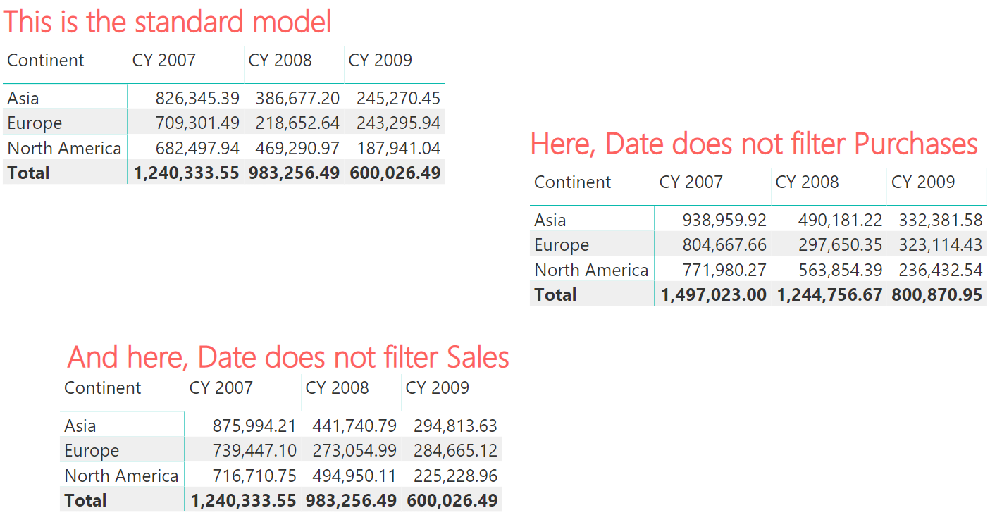
There is no need to comment on each individual number. It is enough to note that the matrices produce three different results. When one of the two relationships is disabled through CROSSFILTER, then Date filters Purchases using path number 2 or 3. When both relationships are active, Date filters Purchases through the combination of all three paths, as I described earlier.

There is a pet name we like to use for these types of models: relationships mazes. The fun part is not in analyzing the numbers; the fun part lies in finding the path that DAX had to discover within the maze to find the exit.

As you noted, this article is not about showing the power of DAX or some interesting algorithm. The goal of this article is to demonstrate how dangerous bidirectional cross-filter relationships are. With a very simple data model containing only five tables, the presence of a bidirectional cross-filter relationship has made the calculations much harder to understand. In the real world where it is common to have models with dozens of tables, the scenario is much harder.

This is the reason we suggest our readers stay away from enabling bidirectional cross-filter relationships in the data model. It is not that bidirectional relationships are bad, or that they are a useless feature. There are a few scenarios where the power of bidirectional cross-filter really shines. However, these need to be leveraged carefully making sure that the model does not become ambiguous because of the bidirectional relationship. Implementing bidirectional cross-filter for the purpose of syncing slicers is definitely a bad idea. After all, if you need to kill ants in the yard, you do not turn on the Death Star.

This is not to say that synced slicers are bad in any way – they are wonderful. It would be great if slicer syncing came as a feature in Power BI implemented through specific queries sent by the client tool, so that users would stop using bidirectional relationships for that purpose.

UPDATE: You can now filter a slicer by using a measure without using a bidirectional filter, read Filter slicers without using bidirectional filters in Power BI for more details.

Next time you are tempted to enable bidirectional cross-filter on a relationship, come back to this article; read it again and take another shot at it, asking yourself again whether you really need that bidirectional cross-filter to be set or not.