Filtering Tables in DAX

If you come from a previous programming or query language, you tend to map your previous knowledge to DAX, forgetting to follow the simpler path of using just the base rules of the language.

I want to show a few examples that – at the beginning – act as mind traps. All of these examples are basic variations of how to filter a table. The numbers we will compute are not meaningful by themselves. The goal is just understanding the theory. Mapping it to real-world examples is left as an interesting exercise for the reader.

Let us start with the following code that returns the same value for all the rows:

DEFINE
    MEASURE Sales[Test] =
        CALCULATE ( 
            SUM ( Sales[Quantity] ), 
            ALL ( 'Product' ) 
        )
EVALUATE
ADDCOLUMNS ( 
    VALUES ( 'Product'[Color] ), 
    "Test", [Test] 
)

The result is this:

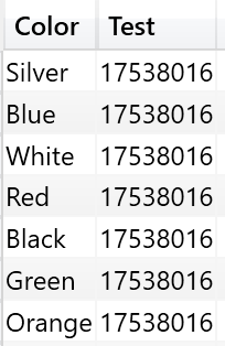
The reason is that ADDCOLUMNS creates a row context on Product[Color], but the measure includes an ALL ( Product ), removing the effect of the filter generated by the context transition. You can obtain a similar effect by performing ALL on the Sales table, instead of the Product one. In fact, if you define the measure as follows:

DEFINE
    MEASURE Sales[Test] =
        CALCULATE ( 
            SUM ( Sales[Quantity] ), 
            ALL ( Sales ) 
        )
EVALUATE
ADDCOLUMNS ( 
    VALUES ( 'Product'[Color] ), 
    "Test", [Test] 
)

The result is – again – the same value repeated for all the rows. While this holds true, most of my students do not really understand why this is happening. In fact, this is the common idea when thinking at how a filter on Product[Color] is used in DAX to filter Sales:

• ADDCOLUMNS filters the Product table, through the Color column.
• The filter on Product[Color] translates in a set of values for the Product[ProductKey] column.
• This set of Product[ProductKey] becomes a filter on Sales[ProductKey], and this filter is applied to the Sales table, resulting in the sales for only the given color.

Said in other words, the filter on Product[Color] becomes a filter on Sales[ProductKey]. Unfortunately, this is not correct. If the latter was true, the following code would return the same value for all the rows, while it does return a different value for each one:

DEFINE
    MEASURE Sales[Test] =
        CALCULATE ( 
            SUM ( Sales[Quantity] ), 
            ALL ( Sales[ProductKey] ) 
        )
EVALUATE
ADDCOLUMNS ( 
    VALUES ( 'Product'[Color] ), 
    "Test", [Test] 
)

You can see the result here:

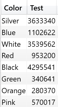
By using ALL on Sales[ProductKey], we get rid of any filter present on Sales[ProductKey], yet the filter on the color remains in place. The reason for this behavior is – indeed – a very simple one: the filter has never been placed on Sales[ProductKey], the filter is only on Product[Color]. If you think – like you would do in a relational database – that the filter works by linking the two tables by the key, you are thinking the wrong way. A further test, if you still don’t trust me, is to try the following:

DEFINE
    MEASURE Sales[Test] =
        CALCULATE (  
            SUM ( Sales[Quantity] ), 
            ALL ( 'Product'[ProductKey] ) 
        )
EVALUATE
ADDCOLUMNS ( 
    VALUES ( 'Product'[Color] ), 
    "Test", [Test] 
)

Again, the result is a different value for every row. Even if you remove the filter from the Product[ProductKey], the filter on Product[Color] remains in place. The point is that the key of the relationship has nothing to share with how filtering works. Filters are defined only by means of using expanded tables (learn more about expanded tables in the previous article Context Transition and Expanded Tables).

The expanded version of Sales contains Product. Thus, when you filter Product[Color], you are directly filtering Sales, with no need to think in terms of relationships, keys, or any other “relational” tool. Because Expanded(Sales) contains Product[Color], filtering Product[Color] filters Sales.

So, why is this measure removing the filter?

DEFINE
    MEASURE Sales[Test] =
        CALCULATE ( 
            SUM ( Sales[Quantity] ), 
            ALL ( Sales ) 
        )
EVALUATE
ADDCOLUMNS ( 
    VALUES ( 'Product'[Color] ), 
    "Test", [Test] 
)

The reason is that this code removes the filter on Product[Color] because it removes any filter from any of the columns in the expanded version of Sales. Remember that – in DAX – when you reference a table in a filter argument, such a table is always expanded. Thus ALL ( Sales ) argument not only removes the filter from any of the native columns of Sales (which – as we have seen – would not have any effect in this case), but it also removes filters from the derived columns of Sales, which include Product[Color]. If you need to convince yourself, you can use ALL including all the columns of Sales, and you will note that the filter on Product[Color] is still in place. The only way to remove it is either to filter the Product table or to use the expanded Sales table.

When activating the bidirectional filtering available in Analysis Services 2016 and Power BI, the scenario becomes a bit more complex. In fact, bidirectional filtering does not work through table expansions. Instead, bidirectional filtering is executed by injecting a direct table filter in a transparent way, when executing the query. This creates the need to take additional care when working with filters.

Consider the following model, where we link Customer to Transactions through the usage of an intermediate dimension (Accounts) and a bridge table (AccountCustomer). In order to make the many-to-many relationship work, we enabled bidirectional filtering on the relationship between the bridge table AccountCustomer and the table Account.

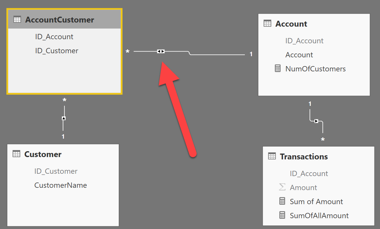
A simple report showing the sum of amount sliced by customer produces the correct result, traversing the many-to-many relationship and generating a result like the following one:

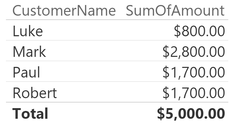
It is worth to recap what is happening here. Customer is filtering the bridge table, and the bridge table, in turn, filters Account, through the bidirectional relationship. As a final step, the Account table filters the Transactions table. Let us be more accurate and speak in terms of expanded tables:

• AccountCustomer expands to Customer. Thus, a filter on the Customer table filters the bridge table, too.
• Transactions expands to Account. Thus, a filter on Account table filters the transactions, too.
• AccountCustomer expands to Account but, in order to activate this kind of filtering, we would need to use the AccountCustomer table as a filter parameter in CALCULATE. We obtain a very similar effect by using the bidirectional filter. The important part, here, is to understand that this filter is not moved through table expansion, but with filter injection.

You can obtain a similar behavior by using the good old method of using the bridge table to move the filter from the many side to the one side, like in the following code:

CALCULATE ( [SumOfAmount], AcccountCustomer ) 

Where SumOfAmount is defined simply as:

SumOfAmount := SUM ( Transactions[Amount] )

Why is this relevant, while speaking about filters? Because, in this case, the filter introduced by the bidirectional filter cannot be removed by simply using ALL on the fact table. In fact, if you author a new measure that removes the filter from Transactions and, thus, from its expanded version (which includes Accounts), the result is not what you would expect. Consider this formula:

SumOfAllAmount = CALCULATE ( [SumOfAmount], ALL ( Transactions ) )

It produces a result identical to the one obtained without ALL :

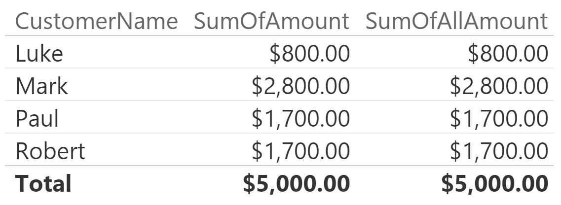
Here the filter is correctly removed from both the Transactions table and the Account one (Account is included in the expanded Transactions). However, the filter on the bridge table is operating on Accounts, through a mechanism that works outside of table expansion. Thus, to remove the filter from the fact table, when it is coming from a bridged dimension, you need to remove the filter from the bridge table too. In fact, the following code results in the filter being removed correctly:

SumOfAllAmount := CALCULATE ( [SumOfAmount], ALL ( AccountCustomer ) )

This picture shows the result of this latter measure:

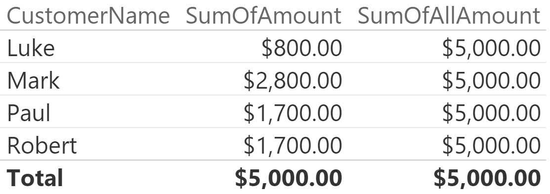
There is no need to remove the filter from either the fact table or the dimension, because their filter is coming, indeed, from the bridge table (actually, from the Account table directly and from the the bridge in an indirect way). Removing the filter from the Account table or from the Transactions table, in this case, proves useless.

As you have seen, at first sight the handling of filters in DAX seems inconsistent, but this is true only if you do not think in terms of expanded tables. The whole DAX relational model is based on expanded tables and, when you grasp the concept, all suddenly makes a lot more sense.