From SQL to DAX: Joining Tables

The SQL language offers the following types of JOIN:

INNER JOIN
OUTER JOIN
CROSS JOIN

The result of a JOIN does not depends on the presence of a relationship in the data model. You can use any column of a table in a JOIN condition.

In DAX there are two ways you can obtain a JOIN behavior. First, you can leverage existing relationships in the data model in order to query data included in different tables, just as you wrote the corresponding JOIN conditions in the DAX query. Second, you can write DAX expressions producing a result equivalent to certain types of JOIN. In any case, not all the JOIN operations available in SQL are supported in DAX.

You can test the examples shown in this article by downloading the sample files (see buttons at the end of the article) and using DAX Studio to run the DAX queries.

Using Relationships in a Data Model

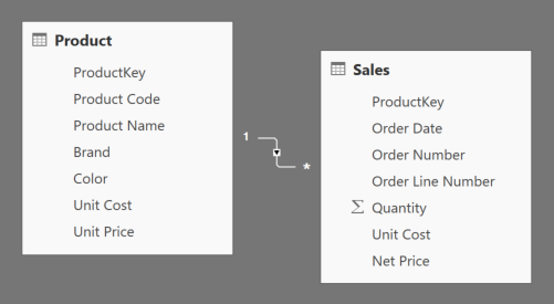
The common approach to obtain a JOIN behavior in DAX is implicitly using the existing relationships. For example, consider a simple model with the tables Sales, Product, and Date. There is a relationship between Sales and each of the other three tables. If you want to see the Quantity of sales divided by Year and Product Color, you can write:

EVALUATE
ADDCOLUMNS (
    SUMMARIZE (
        Sales,
        'Date'[Year],
        Product[Color]
    ),
    "Total Quantity", CALCULATE ( SUM ( Sales[Quantity] ) )
)

The three tables are automatically joined together using a LEFT JOIN between the Sales table (used in the expression for the Total Quantity column) and the other two tables, Date and Product.

SELECT
    d.Year, p.Color, SUM ( s.Quantity ) AS [Total Quantity]
FROM
    Sales s
    LEFT JOIN Date d ON d.DateKey = s.DateKey
    LEFT JOIN Product p ON p.ProductKey = s.ProductKey
GROUP BY
    d.Year, p.Color

Please, note that the direction of the LEFT JOIN is between Sales and Date, so all the rows included in the Sales table that do not have a corresponding row in Date or in Product are grouped in a BLANK value (which corresponds to the concept of NULL in SQL).

If you do not want to aggregate rows, you can simply use RELATED in order to access the columns on lookup tables – on the “one” side of the relationship. For example, consider the following syntax in SQL:

SELECT
    s.*, d.Year, p.Color
FROM
    Sales s
    LEFT JOIN Date d ON d.DateKey = s.DateKey
    LEFT JOIN Product p ON p.ProductKey = s.ProductKey

You obtain the same behavior by using the following DAX query:

EVALUATE
ADDCOLUMNS (
    Sales,
    "Year", RELATED ( 'Date'[Year] ),
    "Color", RELATED ( Product[Color] )
)

You might obtain a behavior similar to an INNER JOIN by applying a filter to the result of the ADDCOLUMNS you have seen so far, removing the rows that have a blank value in the lookup table — assuming that the blank is not a value you might have in the data of that column.

You cannot obtain a CROSS JOIN behavior in DAX by just leveraging relationships in the data model.

Using NATURALLEFTOUTERJOIN and NATURALINNERJOIN with Relationships

Consider these syntaxes in SQL:

SELECT *
FROM a
LEFT OUTER JOIN b
    ON a.key = b.key

SELECT *
FROM a
INNER JOIN b
    ON a.key = b.key

You can write equivalent syntaxes in DAX by using the NATURALLEFTOUTERJOIN and NATURALINNERJOIN functions, respectively, if there is a relationship connecting the two tables involved.

For example, this query returns all the rows in Sales that have corresponding rows in Product, including all the columns of the two tables.

EVALUATE
NATURALINNERJOIN ( Sales, Product )

The following query returns all the rows in Product, showing also the products that have no Sales.

EVALUATE
NATURALLEFTOUTERJOIN ( Product, Sales )

The NATURALLEFTOUTERJOIN and NATURALINNERJOIN functions can also be used with tables that have no relationships – but in this case the columns must not have a data lineage corresponding to physical columns of the data model, as explained later in this article.

Joining Tables without Relationships in DAX

Using CROSSJOIN

Consider this syntax in SQL:

SELECT *
FROM a
CROSS JOIN b

You can write an equivalent syntax in DAX by using the CROSSJOIN function:

EVALUATE
CROSSJOIN ( a, b )

Using NATURALLEFTOUTERJOIN and NATURALINNERJOIN without Relationships

The NATURALLEFTOUTERJOIN and NATURALINNERJOIN functions can join tables that have no relationships, too. In this case, the join condition is based on columns having the same name in the tables involved, but the columns must not have a data lineage corresponding to physical columns of the data model. This can create confusion querying physical tables of a data model.

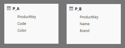
For example, consider two physical tables called P_A (columns ProductKey, Code, and Color) and P_B (ProductKey, Name, and Brand), without any relationship.

You cannot join these two tables by using ProductKey, because these columns have the same name but different data lineages in the model. In fact, the following code generates an error:

EVALUATE
NATURALLEFTOUTERJOIN( P_A, P_B )

The error generated says, “No common join columns detected. The join function ‘NATURALLEFTOUTERJOIN‘ requires at -least one common join column”. A similar message is displayed in case a NATURALINNERJOIN is executed.

In order to join two columns with the same name and no relationships, it is necessary that these columns do not have a data lineage. To obtain that, it is necessary to write the column using an expression that breaks the data lineage, as in the following example.

EVALUATE
VAR A =
    SELECTCOLUMNS (
        P_A,
        "ProductKey", P_A[ProductKey]+0,
        "Code", P_A[Code],
        "Color", P_A[Color]
    )
VAR B =
    SELECTCOLUMNS (
        P_B,
        "ProductKey", P_B[ProductKey]+0,
        "Name", P_B[Name],
        "Brand", P_B[Brand]
    )
VAR Result =
    NATURALLEFTOUTERJOIN ( A, B )
RETURN
    Result

From a performance point of view, a better solution involves the use of TREATAS:

EVALUATE
VAR B_TreatAs =
    TREATAS ( P_A, P_B[ProductKey], P_A[Code], P_A[Color] )
VAR Result =
    NATURALLEFTOUTERJOIN ( B_TreatAs, P_B )
RETURN
    Result

The two solutions share a common goal: providing to the join function in DAX two tables that have one or more columns with the same data lineage. Such column(s) will be used to join the two tables and produce the result.

Using DAX in Excel 2013 and Analysis Services 2012/2014

Former versions of DAX do not have NATURALLEFTJOIN and NATURALINNERJOIN. You can obtain the equivalent of an INNER by embedding the CROSSJOIN expression into a filter, though this is not suggested in case you have to aggregate the result (as will we see later). Consider the following INNER JOIN in SQL:

SELECT *
FROM a
INNER JOIN b ON a.key = b.key

You would write an equivalent syntax in DAX using the following expression:

EVALUATE
FILTER (
    CROSSJOIN ( a, b ),
    a[key] = b[key]
)

There is no simple way of obtaining a syntax in older versions of DAX – up to 2014 – corresponding to a LEFT JOIN in SQL. Nevertheless, you have an alternative if you can assume that you have a many-to-one relationship between the table on the left side and the table on the right side. This was the case of LEFT JOIN using relationships in DAX, and you have seen the solution in DAX using RELATED. If the relationship does not exist, you can use the LOOKUPVALUE function instead.

For example, consider the same SQL query seen previously.

SELECT
    s.*, d.Year, p.Color
FROM
    Sales s
    LEFT JOIN Date d ON d.DateKey = s.DateKey
    LEFT JOIN Product p ON p.ProductKey = s.ProductKey

You can write it in DAX as follows:

EVALUATE
ADDCOLUMNS (
    Sales,
    "Year", LOOKUPVALUE (
        'Date'[Year],
        'Date'[DateKey], Sales[DateKey]
    ),
    "Color", LOOKUPVALUE (
        Product[Color],
        Product[ProductKey], Sales[ProductKey]
    )
)

The version using RELATED is more efficient, but this latter could be a good alternative if the relationship does not exist.
Finally, consider the query that aggregates the result of a LEFT JOIN in SQL, like the one seen previously (we only added the ORDER BY clause):

SELECT
    d.Year, p.Color, SUM ( s.Quantity ) AS [Total Quantity]
FROM
    Sales s
    LEFT JOIN Date d ON d.DateKey = s.DateKey
    LEFT JOIN Product p ON p.ProductKey = s.ProductKey
GROUP BY
    d.Year, p.Color
ORDER BY
    d.Year, p.Color

You can use two approaches here. The first is to leverage the LOOKUPVALUE syntax, aggregating the result as shown in the following DAX syntax:

EVALUATE
SUMMARIZE (
    ADDCOLUMNS (
        Sales,
        "Sales[Year]", LOOKUPVALUE (
            'Date'[Year],
            'Date'[DateKey], Sales[DateKey]
        ),
        "Sales[Color]", LOOKUPVALUE (
            Product[Color],
            Product[ProductKey], Sales[ProductKey]
        )
    ),
    Sales[Year],
    Sales[Color],
    "Total Quantity", CALCULATE ( SUM ( Sales[Quantity] ) )
)
ORDER BY Sales[Year], Sales[Color]

However, if the number of combinations of the aggregated columns is small and the number of rows in the aggregated table is large, then you might consider this approach – verbose, but faster under certain conditions:

DEFINE
    MEASURE Sales[Total Quantity] =
        CALCULATE (
            SUM ( Sales[Quantity] ),
            FILTER (
                ALL ( Sales[ProductKey] ),
                CONTAINS (
                    VALUES ( Product[ProductKey] ),
                    Product[ProductKey], Sales[ProductKey]
                )
            ),
            FILTER (
                ALL ( Sales[DateKey] ),
                CONTAINS (
                    VALUES ( 'Date'[DateKey] ),
                    'Date'[DateKey], Sales[DateKey]
                )
            )
        )
EVALUATE
FILTER (
    ADDCOLUMNS (
        CROSSJOIN ( ALL ( 'Date'[Year] ), ALL ( Product[Color] ) ),
        "Total Quantity", [Total Quantity]
    ),
    NOT ISBLANK ( [Total Quantity] )
)
ORDER BY 'Date'[Year], Product[Color]

Conclusions

In DAX the best way to join tables is always by leveraging physical relationships in the data model, because it results in simpler and faster DAX code. Several techniques are available in DAX in order to join tables. These can be useful for generating calculated tables or small tables in complex expressions that are being used in measures and in calculated columns. However, these techniques are more expensive from a performance point of view and also result in a more complex DAX code.