How to return 0 instead of BLANK in DAX

Power BI mainly uses SUMMARIZECOLUMNS to run queries. SUMMARIZECOLUMNS does not return a row when all the columns computed by the query return BLANK. This behavior is intentional and desirable, as it reduces the number of rows in reports. Despite it being useful and intuitive, sometimes users want to also see rows that produced blanks, because a value of blank (or zero) makes sense in their context.

Indeed, showing that a product did not sell at all and not showing the product at all are two very different things. The former provides an indication of poor performance, whereas the latter hides the information as if it were not relevant. This is not to say that always showing zeroes is a suggestion. In some reports zeroes have meaning, in others they do not. The choice is made by the report author after careful analysis of the requirements.

An example helps in clarifying the concept. We start with a report.

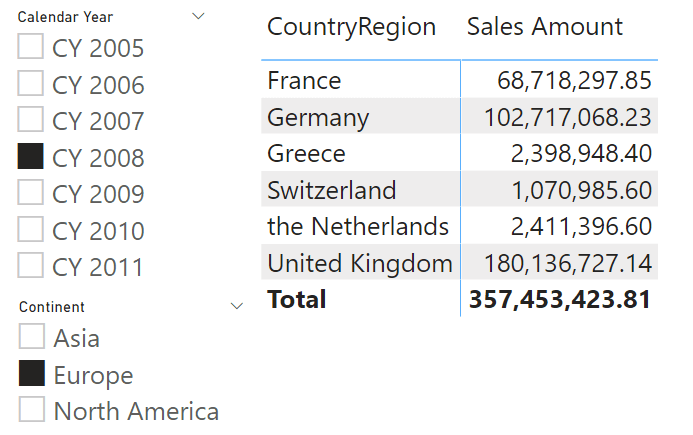
The report is showing the sales amount in different European countries in 2008. Fine, but are there other countries that did not sell? The answer is yes, but the report is not showing them. By removing the filter on the slicer and adding the year on the column of the report, the picture becomes more comprehensive.

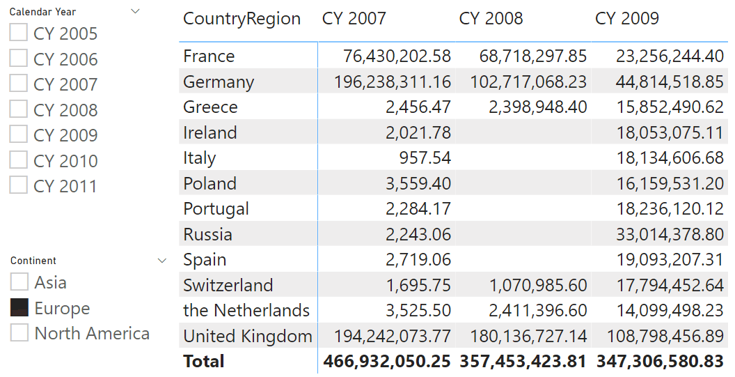
This last report shows that Ireland, Italy and several other countries did not produce any sales in 2008, even though there were sales in 2007 and 2009. As we mentioned, this information may or may not have value but that is not relevant for this article. Here we cover the technique to control the appearance of zeroes instead of blanks. Before we move further, let us elaborate on what we mean by “control”.

Imagine we build a report similar to the reports above but this time at the product level, focusing on Silver cameras and camcorders. There are many products that did not sell in 2008. One is more interesting than the others: Contoso Telephoto Conversion Lens X400 Silver.

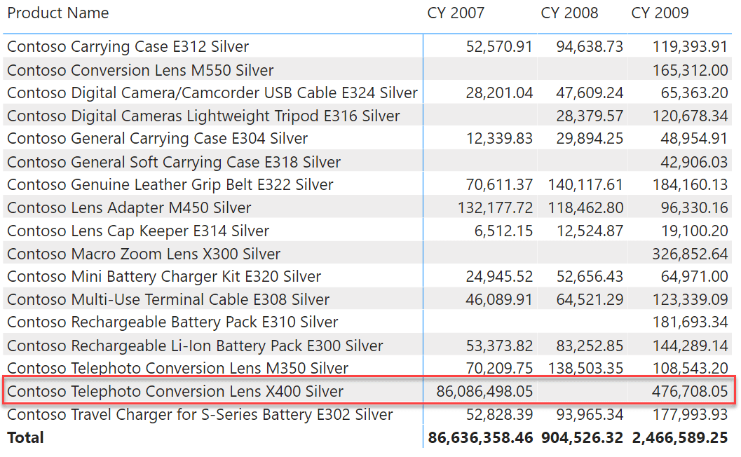
What makes this specific product interesting is that the product sold in 2007, not in 2008 and then it sold again in 2009. Its behavior is different from the other products. Indeed, for most of these products one can argue that they started to sell when they were introduced on the market. Their behavior is quite intuitive: no sales up to a given point in time, then they start selling. We want to highlight this specific product because it shows a gap in sales when it was already present on the market. For other products, we are happy to blank them until their first sale. By doing this, we show gaps when they are real, and we avoid showing non-relevant information – that is, products that could not sell because they were not even available for sale.

Therefore, the requirement is to be able to control when to start showing blanks. In our scenario we control the presence of zeroes based on the product. In your specific scenario, requirements might be different; therefore, you should adapt the technique laid out here to your needs.

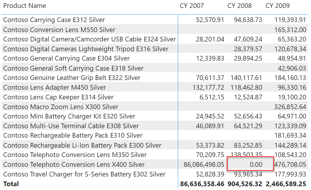
The final report needs to be the following, where you can see the zero for 2008 in the product we highlighted before.

As is always the case, there are multiple solutions to the same scenario. Forcing a value to be zero instead of BLANK is as easy as adding zero to the value. Indeed, BLANK plus zero equals zero. Despite being simple, this solution would show zero for any combination of columns that would result in a blank. For example, it would show zeros for all the years before 2007, or after 2009, just because these years are present in the Date table, despite Sales not containing any row for those years. The solution needs to be more sophisticated than a simple sum.

A pure DAX solution first determines the dates of the first and last transaction in the Sales table. Then, the measure checks whether the current date is in the detected range, in order to decide whether to add the zero or not. Here is a first solution:

SalesZero =
VAR FirstSaleEver =
    CALCULATE ( MIN ( 'Sales'[Order Date] ), ALLEXCEPT ( Sales, 'Product' ) )
VAR LastSaleEver =
    CALCULATE ( MAX ( 'Sales'[Order Date] ), REMOVEFILTERS () )
VAR CurrentDate = MAX ( 'Date'[Date] )
VAR ForceZero = FirstSaleEver <= CurrentDate && CurrentDate <= LastSaleEver  
VAR Amt = [Sales Amount] + IF ( ForceZero, 0 )
RETURN
    Amt

You can change the formula to accommodate various needs. For example, an alternative way of detecting whether to force zero checks whether the currently selected range intersects with the dates between FirstSaleEver and LastSaleEver:

…
VAR ForceZero = FirstSaleEver <= MAX ( 'Date'[Date] ) && MIN ( 'Date'[Date] ) <= LastSaleEver
…

You can choose the formulation that best fits your requirements.

This code runs fast and it works just fine. Still, there is a problem with it. The logic that defines whether a product should show zero or not is based on the Sales table. We determine whether to show a zero or not based on the presence of sales. This detail is basically a negation of our initial requirement: we wanted to be able to control when to show zero independently from Sales Amount. Indeed, if a product were introduced on the market for example on the first of December, we want to start showing zeroes from the first of December even if the first sale of the product were on the 15^th of December. With the current implementation, this is not possible.

A better solution would be to store the information about the starting date in a separate table. If the logic is based on the product only – as it is in our scenario – then a column in the Product table would be just fine. In that case, to determine the starting date to produce zeroes one could use a MIN of the column in Product. In a more complex scenario, you might have more sophisticated rules. For example, the starting date for zeroes might depend on the store, on the country, or on combinations of different dimensions.

In the more generic scenario, the best option is to avoid adding the logic to the DAX code and to rely on a physical table instead. As an example, we created the following table using DAX, even though it is better to create it with Power Query to avoid the danger of circular dependencies:

ZeroGrain = 
VAR MaxSale = MAX ( Sales[Order Date] )
VAR ProdsAndDates = 
    GENERATE ( 
        'Product',
        VAR FirstSaleOfProduct = CALCULATE ( MIN ( 'Sales'[Order Date] ) )
        VAR Dates = DATESBETWEEN ( 'Date'[Date], FirstSaleOfProduct, MaxSale )
        RETURN
            Dates
    )
VAR Result = 
    SELECTCOLUMNS ( 
        ProdsAndDates,
        "ProductKey", 'Product'[ProductKey],
        "Date", 'Date'[Date]
    )
RETURN 
    Result

The table contains one row for each combination of date and product for which we want to show zero instead of BLANK. The table is quite large because it is close to the CROSSJOIN of Product and Date tables. Later in the article, we show how to reduce its size if needed. We need to create relationships with the relevant dimensions. In our case, they are Product and Date.

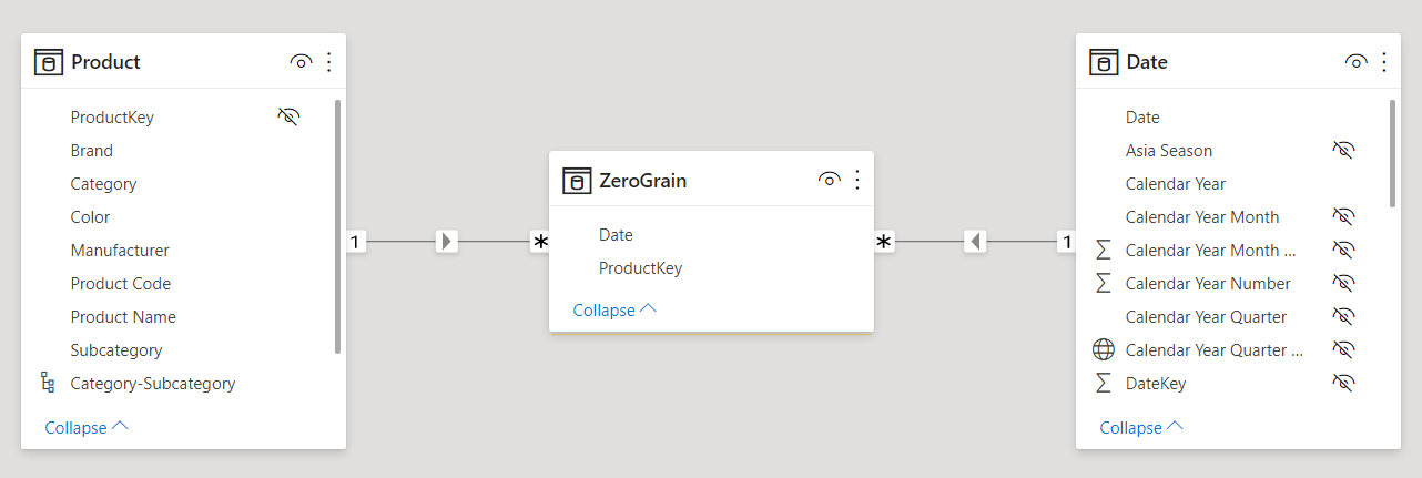
Once the model is completed, the measure no longer needs to perform calculations over dates. This is because the entire logic about when to show zero instead of BLANK is now in the ZeroGrain table. Therefore, the code becomes much simpler:

SalesZeroWithTable = 
VAR ForceZero = COUNTROWS ( ZeroGrain ) > 0
VAR Amt = [Sales Amount] + IF ( ForceZero, 0 )
RETURN
    Amt

 

The result is the very same as the previous measure. The main advantage of using the ZeroGrain table is that the logic to decide whether to show BLANK or zero can now be much more complex. The price, in terms of performance, is due at process time and no longer at query time.

If the size of the ZeroGrain table is too large, you can change its granularity. For example, a good option would be to create the ZeroGrain table at the month granularity instead of the day granularity. By following this path, you reduce the size of the ZeroGrain table but, at the same time, you lose the option of using a regular strong relationship between Date and ZeroGrain. This can be easily solved by relying on a many-to-many cardinality relationship based on the YearMonth column. The increase in complexity due to the many-to-many cardinality relationship is mitigated by the reduced size of the ZeroGrain table and the two options work at comparable speed.

Once implemented for a single measure, this technique can be used to create a calculation group that applies the same logic to any measure. This makes the choice of using BLANK or zero a feature, by using the correct value for the calculation group.

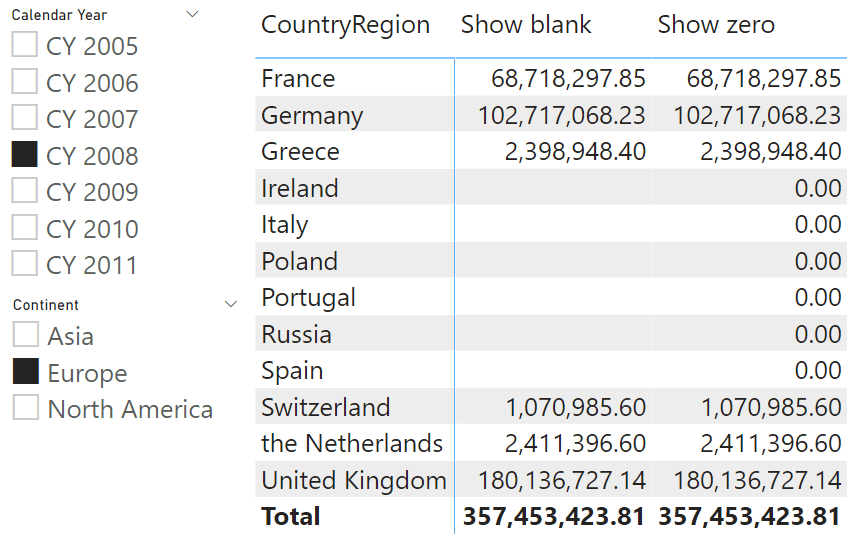
The code of the calculation items is the same as the measure; therefore, we do not show it in the article. If you are interested in the calculation group solution, you can find it in the downloadable content of this article. The result is visible in the next figure, where we used the calculation group on the columns of the report, which is filtering only 2008. You can easily appreciate that when the Show blank calculation item is selected, the result is blank; whereas when Show zero is selected, the countries with no sales show a zero instead.

The choice of which technique to use depends on your specific requirements. For simple scenarios, using the DAX-only solution works just fine. But, if the requirements are complex or if you need more control over when and how to show a zero instead of a blank, then using the ZeroGrain table proves to be an interesting technique to reduce the complexity of your DAX code, and in turn increase the speed of the query.