Numbering sequence of events in DAX

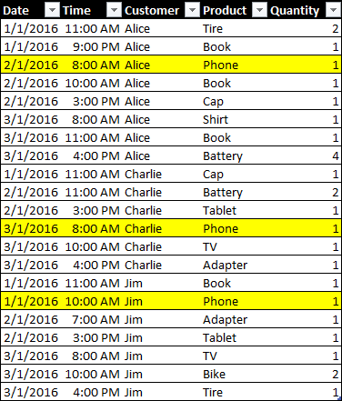
In a model optimized for DAX, you should split date and time in two different columns in order to improve the compression and the usability of the data model. A negative side effect of this design choice is the complexity involved in calculations that have to relate events in sequence. For example, consider this table containing sales of products by date, time, and customer.

If you want to identify the date of the first purchase of a Phone for each customer, you could get the minimum date where the product is Phone for that customer. However, if you want to group the purchases made by a customer before the Phone purchase and those happened after that event, you cannot use just the date, you need to use date and time. Evaluating the minimum date and time of the phone purchase requires a complex (and slow) expression in DAX, unless you create a column containing both date and time, but such approach would be very expensive in terms of storage, because of the reduced compression and the larger dictionary.

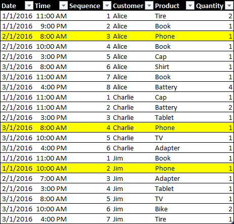
The best solution would be getting a column containing a sequential number for all the purchases made by a customer. Assuming that the data volume of the Sales table depends on the presence of many customers, the range of unique values for this column should be relatively small, if all the customers have a sequence number starting from one. The following table would be the perfect data source.

If you cannot obtain the Sequence column from the data source, because it is not possible or it is too expensive to obtain such information, then you can create a calculated column that evaluates such a number. This is the definition of a DAX calculated column named Sequence by Customer:

Sales[Sequence by Customer] = 
VAR CurrentDate = Sales[Date]
VAR CurrentTime = Sales[Time]
RETURN COUNTROWS ( 
    FILTER ( 
        CALCULATETABLE (
            Sales, 
            ALLEXCEPT ( Sales, Sales[Customer] )
        ),
        Sales[Date] < CurrentDate
          || ( Sales[Date] = CurrentDate 
               && Sales[Time] <= CurrentTime )
    )
)

If you use Excel 2013 or Analysis Service 2012/2014, you should use this version based on EARLIER, because the VAR syntax is available only in following versions of these products:

Sales[Sequence by Customer] =
COUNTROWS ( 
    FILTER ( 
        CALCULATETABLE (
            Sales, 
            ALLEXCEPT ( Sales, Sales[Customer] )
        ),
        ISONORAFTER (Sales[Date], CurrentDate, DESC, Sales[Time], CurrentTime, DESC )
        -- If you use an old Excel version, you do not have ISONORAFTER available
        -- In that case use this corresponding condition:
        -- Sales[Date] < EARLIER ( Sales[Date] )
        --   || ( Sales[Date] = EARLIER ( Sales[Date] ) 
        --        && Sales[Time] <= EARLIER ( Sales[Time] ) )
    )
)

For every row, the FILTER function gets a list of all the rows in Sales for the same customer, and the following expression evaluates the conditions that have to be satisfied for the rows preceding the current one for the same customer. The use of ALLEXCEPT is fundamental in order to avoid any circular reference (http://www.sqlbi.com/articles/understanding-circular-dependencies/) when there is a context transition (in this case generated by CALCULATETABLE) in a calculated column. By counting the number of rows that survive the condition in FILTER you get the desired sequence number for the transactions of the same customer.

Once you have this sequence number, you can easily identify the sequence of the first Phone transaction for every customer. You can create another calculated column using the following DAX expression.

Sales[Sequence First Phone] = 
CALCULATE (
    MIN ( Sales[Sequence by Customer] ),
    ALLEXCEPT ( Sales, Sales[Customer] ),
    Sales[Product] = "Phone"
)

By comparing the two columns, you can segment the transactions executed before and after the first phone purchase made by every customer. Also in this case, we can implement this calculation in a calculated column that will identify the period of the purchase.

Sales[Period] = 
IF ( 
    Sales[Sequence by Customer] < Sales[Sequence First Phone], 
    "0 - Before Phone", 
    IF ( 
        Sales[Sequence by Customer] = Sales[Sequence First Phone], 
        "1 - First Phone", 
        "2 - After First Phone" 
    ) 
)

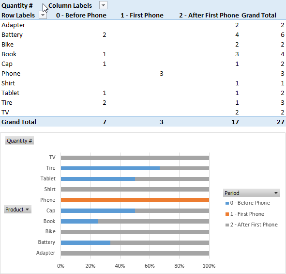
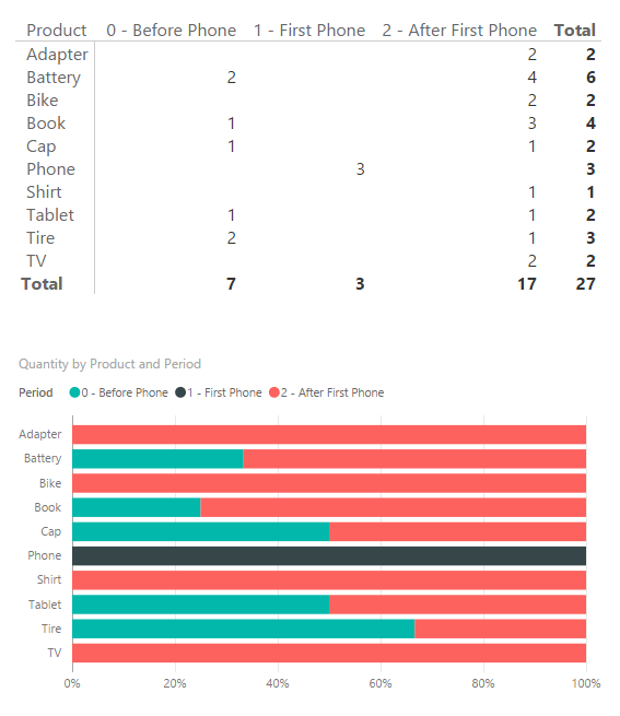
Using the new Period column, you can segment the sales by period, observing whether certain products are sold more frequently before or after the purchase of a Phone. In the following screenshots, you can see the result in both Power Pivot and Power BI.

This technique can be applied to other scenarios where you have a sequence of events that are local to a particular entity (in this case the customer, but it could have been the product, the session in a log file, etc.).

It is important to note the calculated columns described in this article should not be applied to very large tables, because processing such calculated columns could be a very long and memory consuming operation. However, if you have no more than a few million rows in your table, this approach might be more convenient rather than implementing a similar calculation in SQL or Power Query, even if you should consider the hardware available in order to make a final decision.

You can download a ZIP file containing the same example in both Power BI and Excel formats.