Computing an inventory level or an account balance at a given time is a common requirement for many reports. However, when the source data contains all the transactions since the initial zero state, the calculation requires a running sum from the beginning of the data history until the day considered. While easy to implement, a calculation like this can be extremely expensive depending on several factors: the number of cells to compute in the report, the data volume of the transactions, and the cardinality of the dimensions.
The usual approach to optimizing this type of calculation is to introduce a snapshot table that pre-calculates the value of each date for all the dimensions required. Because of the resulting data volume, this solution can be very expensive both in terms of processing time and in terms of resulting memory consumption. A tradeoff is to limit the cardinality of the time available for the snapshot, for example by creating a monthly or quarterly snapshot instead of a daily snapshot. However, this approach limits the analysis of inventory or balance amount trends, and it removes any detail below the snapshot cardinality.
This article shows how to implement a hybrid approach that minimizes the snapshot cost without losing analytical capabilities. This provides outstanding query performance for the reports.
Describing the initial scenario
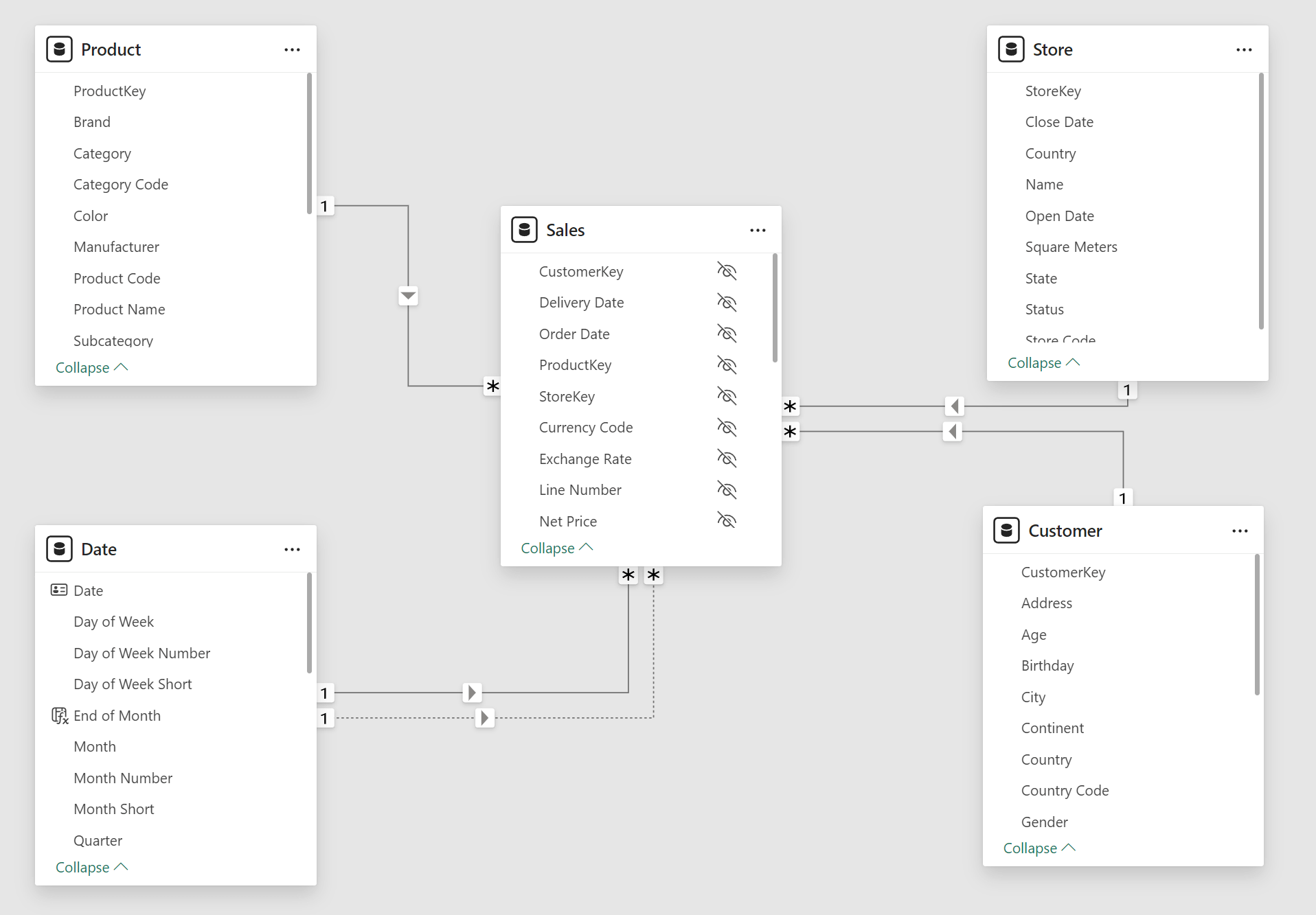
In our model, we have two fact tables that describe the transactions for the Contoso fictitious company. Sales contains the sales transactions data by Date, Product, Customer, and Store.
Supplies tracks the shipments of products delivered to each store by Date, Product, and Store.
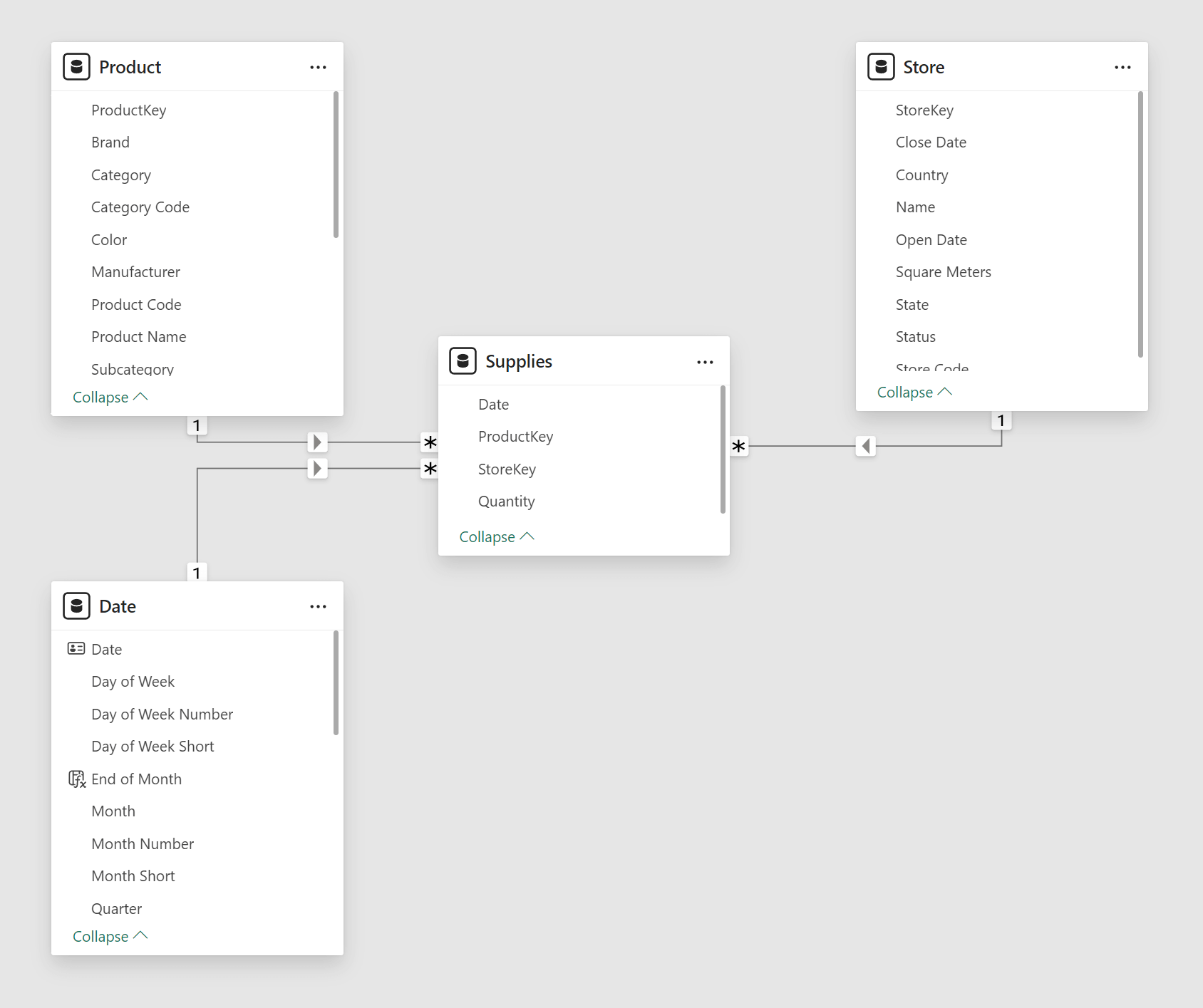
To put it simply, from the perspective of a store, Supplies is what comes in and Sales is what goes out.
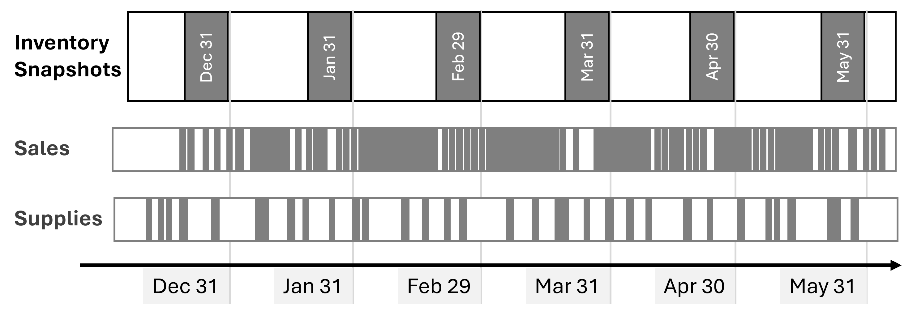
The following picture represents the presence of transactions over time in the Supplies and Sales tables: they have different densities, usually with many transactions for each month.

The actual number of rows depends on the database. In our tests, we used four versions of the Contoso sample database you can download from GitHub: 10K, 100K, 1M, and 10M. The sample file you can download has been processed with the 10K SQL Server database; you can refresh it by changing the connection and using the 100K, 1M, or 10M SQL Server databases. The following are the rows in the model tables: Date covers less than 5 years in 10K and 10 years in the other files, while Product and Store are the same in all the versions.
| Rows in tables | 10K | 100K | 1M | 10M |
| Sales | 7,794 | 199,873 | 2,098,633 | 21,170,416 |
| Supplies | 7,516 | 167,879 | 1,289,555 | 6,390,236 |
| Date | 1,461 | 3,653 | 3,653 | 3,653 |
| Product | 2,517 | 2,517 | 2,517 | 2,517 |
| Store | 74 | 74 | 74 | 74 |
The Qty On Hold measure returns the number of items available on any given date, by subtracting the running sum of Sales[Quantity] from the running sum of Supplies[Quantity]:
Qty On Hold =
VAR LastVisibleDate = MAX ( 'Date'[Date] )
VAR Result =
    CALCULATE (
        SUM ( Supplies[Quantity] ) - SUM ( Sales[Quantity] ),
        'Date'[Date] <= LastVisibleDate
    )
RETURN Result
For any given point in time, the range of dates aggregated for both tables goes from the beginning of the historical data to the date considered. As we will see, this is a slow calculation. The following picture highlights the data aggregated to compute the Qty On Hold for April 20th.

The inventory value is obtained by multiplying the quantity on hold by the product cost. The Amount on Hold measure optimizes that calculation by reducing the iterations to the number of unique Unit Cost values instead of iterating for each Product:
Amount on Hold =
SUMX (
    VALUES ( 'Product'[Unit Cost] ),
    'Product'[Unit Cost] * [Qty On Hold]
)
The performance of this initial scenario is not great. We created two benchmarks: one based on a matrix with different levels of granularity on dates (Year, Month, Date) and another based on a line chart with Date on the X-axis:
// DAX Query for Matrix with three levels (Year, Month, Date)
DEFINE
    VAR __DM3FilterTable =
        TREATAS ( { 2021, 2024 }, 'Date'[Year] )
    VAR __DM5FilterTable =
        TREATAS ( { ( 2021, "Apr 2021" ) }, 'Date'[Year], 'Date'[Year Month Short] )
    VAR __DS0Core =
        SUMMARIZECOLUMNS (
            ROLLUPADDISSUBTOTAL (
                'Date'[Year],
                "IsGrandTotalRowTotal",
                ROLLUPGROUP ( 'Date'[Year Month Short], 'Date'[Year Month Number] ),
                "IsDM1Total",
                NONVISUAL ( __DM3FilterTable ),
                'Date'[Date],
                "IsDM3Total",
                NONVISUAL ( __DM3FilterTable ),
                NONVISUAL ( __DM5FilterTable )
            ),
            // Non-optimized measures
            "Qty_On_Hold", 'Sales'[Qty On Hold],
            "Amount_on_Hold", 'Sales'[Amount on Hold]
        )

EVALUATE
    __DS0Core
ORDER BY
    [IsGrandTotalRowTotal] DESC,
    'Date'[Year],
    [IsDM1Total] DESC,
    'Date'[Year Month Number],
    'Date'[Year Month Short],
    [IsDM3Total] DESC,
    'Date'[Date]
// DAX Query for Line Chart with Date on X-Axis
EVALUATE
SUMMARIZECOLUMNS (
    'Date'[Date],
    "Amount on Hold", 'Sales'[Amount on Hold]
)
ORDER BY 'Date'[Date]
For each benchmark, we also tried a version where we filtered all the stores. This will be useful for performance comparisons with the optimization we will describe later:
// DAX Query for Matrix with three levels (Year, Month, Date)
DEFINE
    VAR __DM3FilterTable =
        TREATAS ( { 2021, 2024 }, 'Date'[Year] )
    VAR __DM5FilterTable =
        TREATAS ( { ( 2021, "Apr 2021" ) }, 'Date'[Year], 'Date'[Year Month Short] )
    VAR __DS0Core =
        SUMMARIZECOLUMNS (
            ROLLUPADDISSUBTOTAL (
                'Date'[Year],
                "IsGrandTotalRowTotal",
                ROLLUPGROUP ( 'Date'[Year Month Short], 'Date'[Year Month Number] ),
                "IsDM1Total",
                NONVISUAL ( __DM3FilterTable ),
                'Date'[Date],
                "IsDM3Total",
                NONVISUAL ( __DM3FilterTable ),
                NONVISUAL ( __DM5FilterTable ),
                FILTER ( ALL ( Store[Country] ), TRUE )
            ),
            // Non-optimized measures
            "Qty_On_Hold", 'Sales'[Qty On Hold],
            "Amount_on_Hold", 'Sales'[Amount on Hold]
        )

EVALUATE
    __DS0Core
ORDER BY
    [IsGrandTotalRowTotal] DESC,
    'Date'[Year],
    [IsDM1Total] DESC,
    'Date'[Year Month Number],
    'Date'[Year Month Short],
    [IsDM3Total] DESC,
    'Date'[Date]
// DAX Query for Line Chart with Date on X-Axis
EVALUATE
SUMMARIZECOLUMNS (
    'Date'[Date],
    FILTER ( ALL ( Store[Country] ), TRUE ),
    "Amount on Hold", 'Sales'[Amount on Hold]
)
ORDER BY 'Date'[Date]
The line chart scenario with the smallest database is already slow (more than 1 second), and it becomes unusable starting from the 100K version of the database.
| Execution time (ms) | 10K | 100K | 1M | 10M |
| Matrix | 57 | 809 | 3,830 | 7,817 |
| Matrix (filtering stores) | 53 | 816 | 3,793 | 7,870 |
| Line Chart | 1,393 | 46,683 | 209,573 | 694,567 |
| Line Chart (filtering stores) | 1,434 | 47,423 | 232,737 | 670,957 |
The slow performance is caused by the running total executed entirely in the formula engine on a large materialization of Sales and Supplies aggregated by Date and Product[Unit Cost]. For example, this is the storage engine query for Sales[Quantity] that returns more than 156,000 rows for the 100K database version (the storage engine query for Supplies[Quantity] is similar):
SELECT
    'Date'[Date],
    'Product'[Unit Cost],
    SUM ( 'Sales'[Quantity] )
FROM 'Sales'
    LEFT OUTER JOIN 'Date'
        ON 'Sales'[Order Date]='Date'[Date]
    LEFT OUTER JOIN 'Product'
        ON 'Sales'[ProductKey]='Product'[ProductKey]
WHERE
    'Date'[Date] IN ( 42959.000000, 43916.000000, 43957.000000, 44914.000000, 44955.000000, 42877.000000, 42918.000000, 43875.000000, 44873.000000, 42795.000000..[3,653 total values, not all displayed] ) ;

Estimated size: rows = 156,803  bytes = 1,881,636
The number of rows materialized depends on the cardinality of the Date and Unit Cost columns for which values are present. The smaller databases do not have data for all the combinations, whereas larger databases cover a more significant percentage of the possible combinations.
Implementing snapshots
To optimize the performance of the query, we need a snapshot table that computes the non-additive measure (Qty On Hold) to avoid any performance degradation in the formula engine. However, we do not want to create a snapshot for every date because the memory cost would be too high. The goal is to use the latest snapshot available for the date considered in a DAX query, and aggregate the remaining transactions in Sales and Supplies after that date to get the correct number for every day. We implement a monthly snapshot at the end of each month.
The first snapshot table is Inventory Store: it has the same cardinality common to Sales and Supplies (Date, Store, and Product); you will find more details about the data volume later in the article.
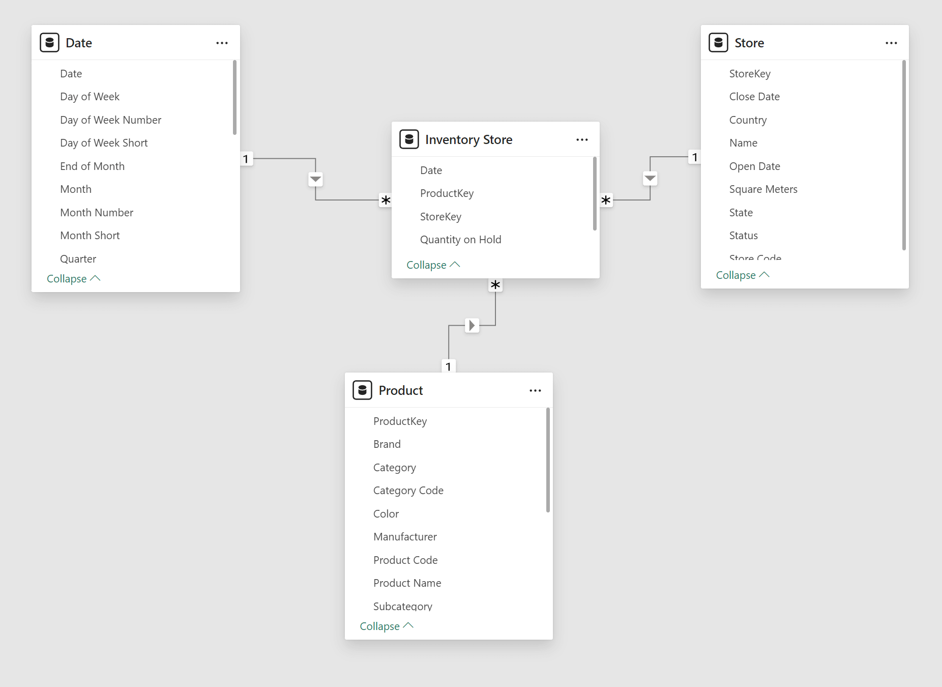
The implementation of the Inventory Store table uses a calculated table. However, this is not an ideal solution for large snapshot tables because the calculated table is calculated every time the model changes and whenever you open the PBIX file. Indeed, if you process the 10M version of the database, opening the processed PBIX file always requires a few minutes! Instead of using DAX, you should consider implementing a snapshot table in SQL or using other ETL tools.
This is the code to compute the Inventory Store table:
Inventory Store =
SELECTCOLUMNS (
    FILTER (
        ADDCOLUMNS (
            CROSSJOIN (
                DISTINCT ( 'Date'[End of Month] ),
                DISTINCT ( 'Product'[ProductKey] ),
                DISTINCT ( Store[StoreKey] )
            ),
            "@Qty",
            VAR InventoryDate = 'Date'[End of Month]
            RETURN
                CALCULATE (
                    SUM ( Supplies[Quantity] ) - SUM ( Sales[Quantity] ),
                    -- Explicit filter with ALLNOBLANKROW to avoid
                    -- circular dependency with relationships
                    FILTER (
                        ALLNOBLANKROW ( 'Date'[Date] ),
                        'Date'[Date] <= InventoryDate
                    )
                )
        ),
        [@Qty] <> 0
    ),
    "ProductKey", 'Product'[ProductKey],
    "StoreKey", Store[StoreKey],
    "Date", 'Date'[End of Month],
    "Quantity on Hold", [@Qty]
)
Because many reports will not require filtering stores, we created a second, smaller snapshot table (Inventory Global) with only the Date and Product cardinality.
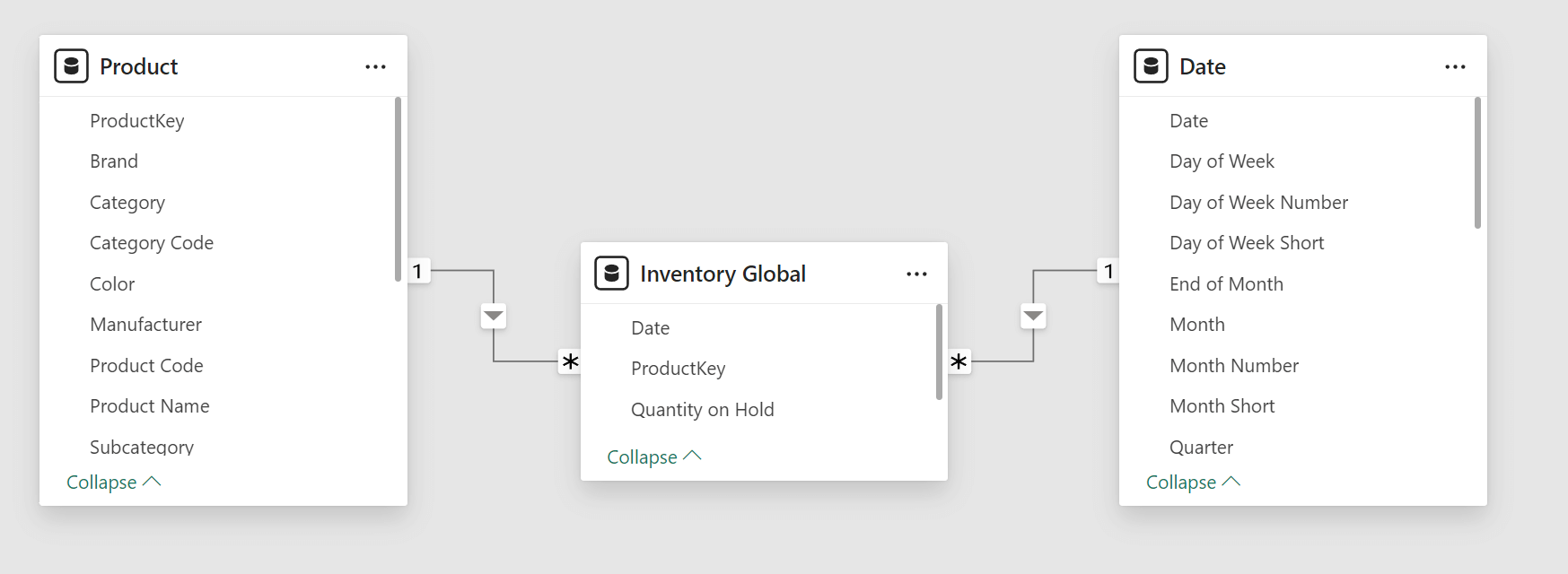
The Inventory Global calculated table is created by aggregating the Inventory Store table:
Inventory Global =
SELECTCOLUMNS (
    SUMMARIZE (
        'Inventory Store',
        'Inventory Store'[Date],
        'Inventory Store'[ProductKey]
    ),
    "Date", 'Inventory Store'[Date],
    "ProductKey", 'Inventory Store'[ProductKey],
    "Quantity on Hold", CALCULATE ( SUM ( 'Inventory Store'[Quantity on Hold] ) )
)
The number of rows for the snapshot tables is smaller than the combined Sales and Supplies tables because, in the sample database, we have several transactions for every period considered in the snapshot. However, the situation depends on the dimension cardinality and the data distribution. You should not make assumptions about your model based on this example – always understand the metrics of your use case!
| Rows in tables | 10K | 100K | 1M | 10M |
| Inventory Store | 13,889 | 290,115 | 2,074,118 | 8,356,391 |
| Inventory Global | 12,171 | 137,664 | 261,292 | 279,211 |
At this point, a measure based on the snapshot alone would look something like this:
CALCULATE (
    SUM ( 'Inventory Store'[Quantity on Hold] ),
    LASTDATE ( 'Date'[Date] )
)
However, a calculation like this would only provide values at the cardinality level of the snapshot table, which we defined for the last day of every month. We need a more complex calculation to take advantage of the snapshot without losing the ability to get the inventory value for any date.
Querying snapshots and hybrid calculations
To retrieve the quantity on hold for any cardinality of Sales and Supplies (Date, Product, and Store), we must implement the following algorithm in a DAX measure:
- Retrieve the last inventory date earlier or equal to the reporting date.
- Retrieve the quantity on hold on that last inventory date.
- Sum Supplies[Quantity] and subtract Sales[Quantity] for all the transaction between the day after the last inventory date and the reporting date.
For example, suppose the reporting date is April 20, 2024. In that case, the measure must sum the Quantity on Hold from the snapshot table on March 31, 2024, add Supplies[Quantity] and subtract Sales[Quantity] by filtering Supplies and Sales between April 1, 2024, and April 20, 2024.
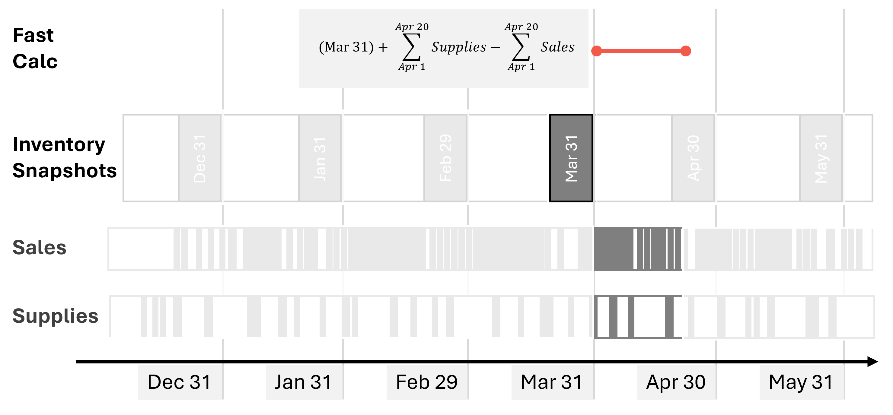
The Qty on Hold (Store) measure implements the algorithm using the Inventory Store snapshot table:
Qty on Hold (Store) =
VAR ReportingDate = MAX ( 'Date'[Date] )
VAR LastInventoryDate =
    CALCULATE (
        MAX ( 'Inventory Store'[Date] ),
        REMOVEFILTERS(),
        'Date'[Date] <= ReportingDate
    )
VAR LastInventoryQuantity =
    CALCULATE (
        SUM ( 'Inventory Store'[Quantity on Hold] ),
        'Date'[Date] = LastInventoryDate
    )
VAR LastTransactionsQuantity =
    CALCULATE (
        SUM ( Supplies[Quantity] ) - SUM ( Sales[Quantity] ),
        'Date'[Date] > LastInventoryDate
            && 'Date'[Date] <= ReportingDate
    )
VAR Result =
    LastInventoryQuantity + LastTransactionsQuantity
RETURN Result
By using Qty on Hold (Store) for the line chart scenario, the query execution is from 3 to 71 times faster, depending on the model.
| Execution time (ms) | 10K | 100K | 1M | 10M |
| Line Chart (no snapshot) | 1,434 | 47,423 | 232,737 | 670,957 |
| Line Chart (Store snapshot) | 471 | 3,661 | 6,149 | 9,445 |
| Improvement | 3x | 13x | 38x | 71x |
For educational purposes, we also implemented a second snapshot table (Inventory Global) with a lower granularity. With the data volume and the cardinality of our examples, this second snapshot is not necessary, but in larger models you might consider multiple, smaller snapshot tables to further optimize the query response time for queries that do not filter across all the dimensions.
The measure to obtain the quantity on hold based on the Inventory Global snapshot is very similar to the one used for Inventory Store:
Qty on Hold (Global) =
VAR ReportingDate = MAX ( 'Date'[Date] )
VAR LastInventoryDate =
    CALCULATE (
        MAX ( 'Inventory Global'[Date] ),
        REMOVEFILTERS(),
        'Date'[Date] <= ReportingDate
    )
VAR LastInventoryQuantity =
    CALCULATE (
        SUM ( 'Inventory Global'[Quantity on Hold] ),
        'Date'[Date] = LastInventoryDate
    )
VAR LastTransactionsQuantity =
    CALCULATE (
        SUM ( Supplies[Quantity] ) - SUM ( Sales[Quantity] ),
        'Date'[Date] > LastInventoryDate
            && 'Date'[Date] <= ReportingDate
    )
VAR Result =
    LastInventoryQuantity + LastTransactionsQuantity
RETURN Result
By using Qty on Hold (Global) for the line chart scenario, the improvement in the execution time of the query is very similar to the other larger snapshot – the differences are within the range of tolerance between different executions.
| Execution time (ms) | 10K | 100K | 1M | 10M |
| Line Chart (no snapshot) | 1,393 | 46,683 | 209,573 | 694,567 |
| Line Chart (Global snapshot) | 468 | 3,763 | 5,942 | 9,405 |
| Improvement | 3x | 12x | 35x | 74x |
In the database we are using for our tests, we do not have a reason to justify two snapshot tables: we could use the one with the larger cardinality (Inventory Store) for any query. However, we want to describe how to create a single measure that automatically chooses the best snapshot available to maximize performance at the cardinality level of each query.
Choosing between multiple snapshot tables
The Qty on Hold (Store) and Qty on Hold (Global) measures are hidden because we want to exhibit a single measure that automatically chooses the smaller snapshot table compatible with the cardinality of the query. In this scenario, if the query places a filter on the Store table, then the Inventory Store table should be used – otherwise, Inventory Global can provide the same result by querying a smaller table. A direct approach could be the following:
IF (
    ISCROSSFILTERED ( 'Store' ),
    [Qty on Hold (Store)],
    [Qty on Hold (Global)]
)
However, you must maintain the code of this measure if the cardinality of the snapshot tables changes. An example of this is when new dimension tables are added to the data model and related to one or more snapshot tables. If we assume that a snapshot (Inventory Global) has a subset of the cardinality of another snapshot (Inventory Store) and that the relationships between snapshots and dimensions are all regular one-to-many, then we can use the following pattern to decide which snapshot to use:
IF (
    CALCULATE (
        ISCROSSFILTERED ( <full snapshot> ),
        REMOVEFILTERS ( <subset snapshot> ),
    ),
    <use full snapshot>,
    <use subset snapshot>
)
The pattern leverages the fact that REMOVEFILTERS removes the filter from the expanded table of <subset snapshot>, leaving only filters on dimensions that are not connected to the <subset snapshot> table. ISCROSSFILTERED returns TRUE if any of those filters are present and <full snapshot> must be used; otherwise, it returns FALSE and the <subset snapshot> table can be used.
Therefore, we can write the optimized Qty on Hold (opt.) measure this way:
Qty on Hold (opt.) =
IF (
    CALCULATE (
        ISCROSSFILTERED ( 'Inventory Store' ),
        REMOVEFILTERS ( 'Inventory Global' )
    ),
    // Filter detail below Global
    [Qty on Hold (Store)],
    [Qty on Hold (Global)]
)
We also create an optimized version of Amount on Hold which we call Amount on Hold (opt.). It uses Qty on Hold (opt.):
Amount on Hold (opt.) =
SUMX (
    VALUES ( 'Product'[Unit Cost] ),
    'Product'[Unit Cost] * [Qty on Hold (opt.)]
)
We tested the Amount on Hold (opt.) measure in the Matrix scenario: the increased number of storage queries slightly slows down the performance of the smaller model (10K), whereas for the other models the improvement ranges from 7 to 42 times faster.
| Execution time (ms) | 10K | 100K | 1M | 10M |
| Matrix (no snapshot) | 53 | 816 | 3,793 | 7,870 |
| Matrix (optimized with snapshot) | 64 | 120 | 157 | 187 |
| Improvement | 0.8x | 7x | 24x | 42x |
Additional optimizations
Section added on 2025-01-16. A smart reader (see “zenzei” in the comments section) noticed that there is an additional optimization possible for the Amount on Hold measure. We focused too much on improving the Quantity calculation and forgot to show that – if the measure does not have other complexities – removing the materialization from the context transition is extremely helpful, even if this means losing the central definition of Quantity as business calculation. Because it is just the sum of a column, here is a faster version of Amount on Hold that does not rely on the existing Quantity measure.
The following measure does not use any snapshot and – in this simple example – outperforms the snapshot versions.
MEASURE Sales[Amount on Hold (opt.2)] =
    VAR LastVisibleDate = MAX ( 'Date'[Date] )
    VAR Result =
        CALCULATE (
            SUMX ( Supplies , RELATED ( 'Product'[Unit Cost] ) * Supplies[Quantity] )
                - SUMX ( Sales, RELATED ( 'Product'[Unit Cost] )  * Sales[Quantity] ),
            'Date'[Date] <= LastVisibleDate
        )
    RETURN result
However, whenever this approach is not possible – or when the data volume of Sales and Supplies requires using a snapshot anyway, then all the techniques described in the report still apply.
As usual, do your own benchmark and evaluate which option provides good performance for your requirements. With similar benchmark, remember that the simpler the better!
Conclusions
Snapshot tables can improve the performance of calculating running totals like the inventory amount. Balancing the memory and the processing time required for the snapshot tables with the query performance improvement requires a hybrid approach that aggregates the transactions following the last available snapshot. In case multiple snapshots are required to maximize the performance of high-level aggregations in very large models, you can choose the snapshot to use by inspecting the filter context with ISCROSSFILTERED – this relies on techniques that require a small amount of DAX code, and that the engine can optimize well.
 Marco Russo & Alberto Ferrari