A virtual relationship is a DAX pattern to transfers a filter context from a table to another, simulating the behavior of a physical relationship defined in the data model. This technique is useful whenever a relationship does not exist, or when it cannot be created because the relationship is not a one-to-many, or because it is defined by two or more columns. You can find a longer description in the article Physical and Virtual Relationships in DAX.
Just to recap, we have two patterns in DAX to manage virtual relationships. The first is based on FILTER, and it works on any version of DAX.
[Filtered Measure] :=
CALCULATE (
    <target_measure>,
    FILTER (
        ALL ( <target_granularity_column> ),
        CONTAINS (
            VALUES ( <lookup_granularity_column> ),
            <lookup_granularity_column>,
            <target_granularity_column>
        )
    )
)
The second is based on INTERSECT, and it works on Excel 2016, Power BI, and SSAS Tabular 2016.
[Filtered Measure] :=
CALCULATE (
    <target_measure>,
    INTERSECT (
        ALL ( <target_granularity_column> ),
        VALUES ( <lookup_granularity_column> )
    )
)
The February 2017 version of Power BI Desktop introduced a new DAX function, called TREATAS, which will appear in future version of Analysis Services and Excel.
[Filtered Measure] :=
CALCULATE (
    <target_measure>,
    TREATAS (
        VALUES ( <lookup_granularity_column> ),
        <target_granularity_column>
    )
)
If you are used to the INTERSECT pattern, you might find the TREATAS syntax strange, because you must invert the arguments: the first one is the filter context to read, the second one includes the columns. You can also use TREATAS with two or more columns. For example, this is the pattern for a virtual relationship using INTERSECT:
[Filtered Measure] :=
CALCULATE (
    <target_measure>,
    INTERSECT (
        ALL (
            <target_granularity_column_1>,
            <target_granularity_column_2>
        ),
        SUMMARIZE (
            <lookup_table>
            <lookup_granularity_column_1>
            <lookup_granularity_column_2>
        )
    )
)
The same result can be obtained using TREATAS:
[Filtered Measure] :=
CALCULATE (
    <target_measure>,
    TREATAS (
        SUMMARIZE (
            <lookup_table>
            <lookup_granularity_column_1>
            <lookup_granularity_column_2>
        ),
        <target_granularity_column_1>,
        <target_granularity_column_2>
    )
)
The rules of thumb for using these patterns are:
- Always use a physical relationship to propagate filters whenever possible.
- If you cannot use a physical relationship, you should implement a virtual relationship using TREATAS.
- Only use the INTERSECT pattern if TREATAS is not available in the DAX version you use.
- Only use the FILTER pattern if TREATAS and INTERSECT are not available in the DAX version you use.
If the granularity of the filter propagated is relatively small, you might consider a virtual relationship as a possible alternative to a physical one. The slower performance of a virtual relationship shouldn’t impact the overall execution time in a visible way, but remember that your experience might vary depending on the complexity of the query.
Let’s see in the following examples why you should follow these rules.
Relationships with multiple columns
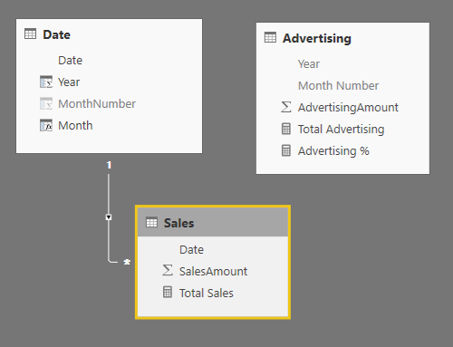
Consider a model where the Sales table has a day granularity, whereas the table Advertising has a month granularity. (This is the file “Day and Month Granularity – Without Relationships.pbix” in the samples you can download.) You cannot create a physical relationship between Date and Advertising, because the granularity is defined by two columns (Year and Month Number), and there are multiple rows with the same combination of year and month in the Date table.
If you want to compare the sum of SalesAmount and AdvertisingAmount for each month, you need to propagate the filter context from Date to Advertising. You can define the Total Advertising measure using the TREATAS function to perform this filter propagation.
[Total Advertising] :=
CALCULATE (
    SUM ( Advertising[AdvertisingAmount] ),
    TREATAS (
        SUMMARIZE ( 'Date', 'Date'[Year], 'Date'[MonthNumber] ),
        Advertising[Year],
        Advertising[Month Number]
    )
)
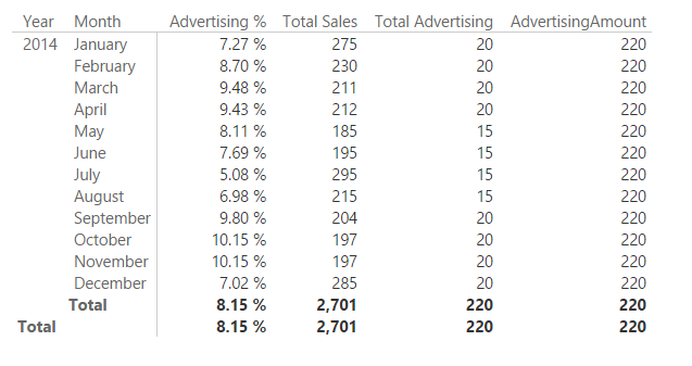
In the following picture, you see that the Total Advertising computes a correct computation month by month, whereas the column AdvertisingAmount simply sums the value of the corresponding column for all the rows in Advertising, because there is no filter propagation between Date (which has a month selected in every row of the report) and Advertising.
If the granularity is small (up to hundreds of values), this approach is probably good enough. However, if you have a higher number of unique values propagated in a virtual relationship, then you should consider an approach based on a physical relationship. In a simple one-to-many relationship, you can just combine different columns into a single one. If the relationship is a many-to-many, you can implement the pattern described in the article Many-to-many relationships in Power BI and Excel 2016. You can find an example of this approach in the file “Day and Month Granularity – With Relationships” in the samples you can download.
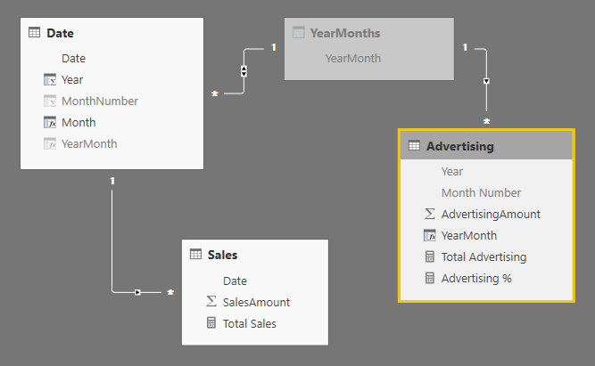
In the following diagram, you see that the bridge table YearMonths is connected to the calculated column YearMonth defined in the two tables Date and Advertising. The bidirectional filter enabled between YearMonths and Date guarantees that the filter context propagates from Date to YearMonth, and then it also goes to Advertising because of the one-to-many relationship between YearMonths and Advertising.
The YearMonth calculated column simply combines year and month number in a single value.
Advertising[YearMonth] = Advertising[Year] * 100 + Advertising[Month Number]
The YearMonths calculated table is defined as follows, getting the list of unique values of YearMonth from the date table Date.
YearMonths = ALL ( 'Date'[YearMonth] )
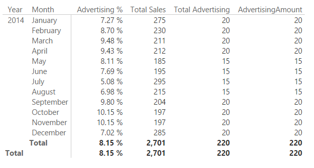
At this point, the Total Advertising measure can be defined using a simple SUM aggregation. In fact, the result of Total Advertising now corresponds to the result of the column AdvertisingAmount in the report, which implicitly aggregates the corresponding column in the Advertising table using the SUM aggregation function.
The approach based on a physical relationship is usually better in terms of performance. However, it requires the relationship to be defined in the data model. Sometime this is not possible, for example because you are querying a model that you do not control, or because in a complex model the presence of additional relationships would generate circular references or other undesired side effects of the filter propagation. This was not the case of the simple data model used as an example.
Cost of virtual relationships
You have seen that the best practice is to always use a physical relationship whenever possible. This is because the cost of a relationship depends on the cardinality of the filter propagated. A relationship based on a column with 100 unique values is usually faster than another one based on 1,000,000 unique values. This problem is described in more details in the article Costs of Relationships in DAX. This section compares the performance of different implementations of a virtual relationship with the corresponding solution based on a physical relationship.
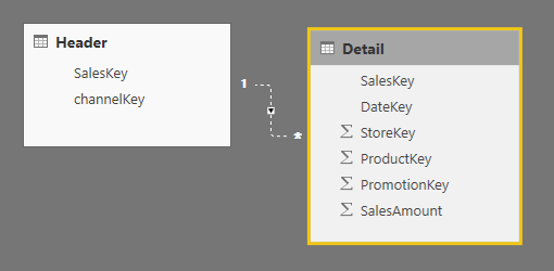
The file “HeaderDetail.pbix” in the samples you can download has a simple schema with two tables, Header and Detail. The SalesKey column uniquely identify each row in the Header table, and it has an inactive one-to-many relationship to the Detail table. (In reality, in the sample data the Detail table has only one for each Header row, but this is not relevant for the performance comparison of this test.)
In the queries used to evaluate the performance, we will make the relationship active only to measure the performance of the physical relationship, whereas it will be ignored by testing the different approaches using virtual relationship. The test simply aggregates the SalesAmount column grouping the result by channelKey. What makes this test meaningful is the cardinality of the SalesKey column, which has 3,406,089 rows. In other words, we are simulating the scenario of a large dimension by using the smallest possible data model.
If you want to replicate these tests on your own machine, open the HeaderDetails.pbix file, then start DAX Studio and connect it to Power BI Destkop.
Virtual relationship using FILTER
The virtual relationship using the FILTER technique is implemented using the following query.
EVALUATE
CALCULATETABLE (
    SUMMARIZECOLUMNS (
        Header[channelKey],
        "Sales", CALCULATE (
            SUM ( Detail[SalesAmount] ),
            FILTER (
                ALL ( Detail[SalesKey] ),
                CONTAINS (
                    VALUES ( Header[SalesKey] ),
                    Header[SalesKey], Detail[SalesKey]
                )
            )
        )
    )
)
This is the slowest approach:
- Total: 14,787 ms
- FE: 12,319 ms
- SE: 2,468 ms
- 3 SE queries:
- 3,406,089 rows / 13,306 KB
- 3,406,089 rows / 13,306 KB
- 3,406,089 rows / 39,916 KB
Virtual relationship using INTERSECT
The approach using INTERSECT has a simpler DAX syntax.
EVALUATE
CALCULATETABLE (
    SUMMARIZECOLUMNS (
        Header[channelKey],
        "Sales", CALCULATE (
            SUM ( Detail[SalesAmount] ),
            INTERSECT (
               ALL ( Detail[SalesKey] ),
               VALUES ( Header[SalesKey] )
            )
        )
    )
)
The performance is slightly better, but the advantage is limited to an improved query plan in the formula engine, without reducing the redundant materializations required by this approach:
- 3,406,089 rows / 13,306 KB
- 7 rows / 1 KB
- 3,406,089 rows / 13,306 KB
- 3,406,089 rows / 39,916 KB
Virtual relationship using TREATAS
The approach using TREATAS is not much different to INTERSECT, besides the syntax and the order of arguments:
EVALUATE
CALCULATETABLE (
    SUMMARIZECOLUMNS (
        Header[channelKey],
        "Sales", CALCULATE (
            SUM ( Detail[SalesAmount] ),
            TREATAS ( VALUES ( Header[SalesKey] ), Detail[SalesKey] )
        )
    )
)
The performance is the best one for a virtual relationship, mainly because this approach reduces the storage engine workload from three large materialization to only two, and this also improves the performance of the formula engine:
- 3,406,089 rows / 13,306 KB
- 3,406,089 rows / 39,916 KB
Physical relationship
The physical relationship is the best approach. The query simply activates the existing relationship.
EVALUATE
CALCULATETABLE (
    SUMMARIZECOLUMNS (
        Header[channelKey],
        "Sales", SUM ( Detail[SalesAmount] )
    ),
    USERELATIONSHIP ( Detail[SalesKey], Header[SalesKey] )
)
This approach provides the best performances, because it removes the need of materializing a large number of rows that must be computed by the formula engine. The join between the two tables and the aggregation is entirely computed by the storage engine, obtaining an improvement of two orders of magnitude.
- 7 rows / 1 KB
Performance comparison
In the following table, you can see a comparison of the execution time between the different techniques.
| Relationship Type | Execution | Comparison with Physical Relationship | Improvement over Virtual FILTER (%) |
| Virtual – FILTER | 14,787 | 137x | |
| Virtual – INTERSECT | 12,920 | 120x | -13% |
| Virtual – TREATAS | 7,464 | 69x | -50% |
| Physical | 108 | 1x | -99% |
Using TREATAS you can run a query in 50% of the time required by the FILTER approach, whereas INTERSECT has only a marginal improvement (13%). TREATAS is the clear choice when you implement a virtual relationship, but you can also see that with a large dimension the advantage of a physical relationship is huge. These differences are barely measurable for relationships with a low granularity, making the virtual relationship a possible option in those cases.
You should run similar tests on your own model to verify that the virtual relationship has a cost that you can afford (the advantage is that it has no impact on the data model).
Arbitrary shaped filters
When you define an arbitrary shaped filter, the TREATAS function has flexibility and efficiency that is harder to obtain using INTERSECT. For example, you can write this calculation to retrieve the quantity of Blue products sold in France plus the Green products sold in Ireland.
EVALUATE
SUMMARIZECOLUMNS (
    'Date'[Calendar Year],
    "Quantity", CALCULATE (
        SUM ( Sales[Quantity] ),
        TREATAS (
            { ( "Blue", "France" ), ( "Green", "Ireland" ) },
            'Product'[Color],
            Customer[Country]
        )
    )
)
Creating such an arbitrary filter using columns of different tables is much more expensive. The simpler syntax using INTERSECT is not very efficient if compared to the TREATEAS one:
EVALUATE
SUMMARIZECOLUMNS (
    'Date'[Calendar Year],
    "Quantity", CALCULATE (
        SUM ( Sales[Quantity] ),
        INTERSECT (
            CROSSJOIN (
                ALL ( Product[Color] ),
                ALL ( Customer[Country] )
            ),
            { ( "Blue", "France" ), ( "Green", "Ireland" ) }
        )
    )
)
Using the CROSSJOIN you materialize a table that is not required. You can optimize this by filtering only the two colors and two countries upfront, so the CROSSJOIN only materializes four combinations, but the entire process is removed by using TREATAS, which creates an arbitrary filter that is pushed to the storage engine in a direct way, without having to materialize a table in advance. This could result in much better performance in scenarios where an arbitrary shaped filter is required, especially when you combine columns from different tables.
Conclusion
The TREATAS function is the best way to implement a virtual relationship. This approach is good if you have a small number of unique values to propagate in the filter. However, you should always consider that a physical relationship can provide an improvement of one or two order of magnitudes for a high cardinality relationship. In complex data models, the virtual relationship could be the only option, because additional physical relationships might have undesired side effects in the filter propagation to other tables.
Returns a table that has been filtered.
FILTER ( <Table>, <FilterExpression> )
Returns the rows of left-side table which appear in right-side table.
INTERSECT ( <LeftTable>, <RightTable> )
Treats the columns of the input table as columns from other tables. For each column, filters out any values that are not present in its respective output column.
TREATAS ( <Expression>, <ColumnName> [, <ColumnName> [, … ] ] )
Adds all the numbers in a column.
SUM ( <ColumnName> )
Returns a table that is a crossjoin of the specified tables.
CROSSJOIN ( <Table> [, <Table> [, … ] ] )
 Marco Russo