Understanding apply semantics for window functions in DAX

Find more in the Understanding Visual Calculations in DAX whitepaper available to SQLBI+ subscribers

Window functions like OFFSET and WINDOW return rows from a table based on the current row. For example, OFFSET (-1) returns the previous row. The main question is: how does OFFSET determine the current row? Intuitively, it searches in the row context and in the filter context for values of columns, and it determines the current row. Unfortunately, that intuitive understanding is missing many details. Although it is easy to intuit the current row in simple queries, things are sometimes more complex. To make sense of the current row in a non-trivial scenario, you need to understand apply semantics.

For example, look at the following query:

EVALUATE
SUMMARIZECOLUMNS (
    Product[Brand],
    "Sales", [Sales Amount],
    "Test",
        CALCULATE (
            [Sales Amount],
            OFFSET (
                -1,
                ORDERBY ( Product[Brand] )
            )
        )
)

SUMMARIZECOLUMNS groups by Brand, and the Test measure returns the value of the previous brand in alphabetical order because of the ORDERBY clause used in OFFSET.

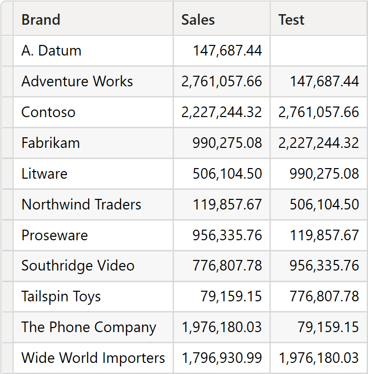
However, by changing the way ORDERBY sorts data, the result is much more complex to figure out:

EVALUATE
SUMMARIZECOLUMNS (
    Product[Brand],
    "Sales", [Sales Amount],
    "Test",
        CALCULATE (
            [Sales Amount],
            OFFSET (
                -1,
                ORDERBY ( 'Date'[Year] )
            )
        )
)

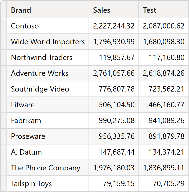
OFFSET is expected to return to the previous year, whereas in the previous query it was returning the previous brand. Unfortunately, the query is not grouping by year. Therefore, what is the meaning of the previous year if no current year is filtered? Despite this issue, the query runs, and it returns a value. However, understanding what the value represents requires some level of effort.

We first outline the apply semantics algorithm; then, we run a couple of examples to verify the behavior of apply semantics in more detail.

The algorithm aims to find the current row(s) in the source table. The source table contains both model columns (columns with the lineage of a column in the model) and local columns (for example, columns added with ADDCOLUMNS, with no lineage). The apply semantics algorithm is rather simple and consists of two separate steps: matching and apply. The two steps operate on the two different types of columns, model columns and local columns.

Matching

Matching applies only to model columns; local columns are used later. During matching, the algorithm determines the possible values for each column in the model. At the end of the matching process, each model column is matched with a set of possible values.

Each model column of the source table is searched for in the row contexts. If the column is present in a row context, it is matched with the only value of that row context. If multiple nested row contexts exist within the same column, the engine uses the innermost row context. If a column matches the row context, its value is unique and well defined.

If a model column is not matched with any row context, then the VALUES of the column are evaluated in the current filter context, and the column itself is matched with the result of VALUES. This step might generate multiple values because a column can show multiple values in the filter context. The model column is matched with all the values discovered.

Please note that multiple columns may be considered during this step, each of which can have multiple values. The full CROSSJOIN of all the possible values of all columns is generated (there is no auto-exist). Hence, the more model columns in the source table, the larger the set of options to scan.

At the end of the matching process, all model columns of the source table are bound to their possible values. The result of the matching process is a table containing all the possible combinations of values of the model columns in the source table. This table does not contain local columns; therefore, it contains fewer columns than the window function source table and most likely a different number of rows. We call the result of the binding process the Matching Table.

Developers can use the MATCHBY modifier to define which columns must be used during the matching process. Please note that MATCHBY can only be used with model columns.

Apply

Once matching has occurred, the engine creates the matching table, which is a table of candidates for the current row. However, the matching table is missing the local columns, and it most likely includes combinations of values for the model columns that might not be present in the source table. DAX uses the matching table to filter the source table to add the local columns and to obtain the list of current rows. The source table filtered by the matching table contains all the columns of the source table: both model columns and local columns. Besides, it contains only rows that do exist in the source table. Therefore, it is a set of valid rows in the source table.

The set of rows created with this second step is the Apply Table. The apply table contains the set of rows of the source table that are considered the “current” row for apply semantics. The window function is then executed once per row in the apply table, and the execution results are union-ed together to generate the result.

Pseudo-DAX Algorithm

The following is pseudo-DAX code to make the steps of “apply semantics” clearer. Be mindful that we are not using real DAX functions. Our goal is only to show you the execution flow:

EVALUATE
VAR MatchingTable = 
    MATCH ( 
       SourceTable, 
       Evaluation Contexts 
    )
VAR ApplyTable = 
    FILTER ( 
        SourceTable,
        (Matched Columns in SourceTable) IN MatchingTable
    )
VAR Result = 
    DISTINCT ( 
        SELECTCOLUMNS ( 
            GENERATE ( 
                ApplyTable,
                <Result of Window Function>
            ),
            <All columns in the Source table>
        )
    )
RETURN
    Result

The GENERATE function in DAX implements the SQL APPLY statement. Hence the name, Apply Semantics.

Apply semantics example (1)

Let us look at the algorithm with the following example:

EVALUATE
SUMMARIZECOLUMNS (
    Customer[Continent],
    TREATAS ( { 2018, 2019 }, 'Date'[Year] ),
    "Sales", [Sales Amount],
    "Sales PY",
        CALCULATE (
            [Sales Amount],
            OFFSET (
                -1,
                SUMMARIZE ( ALL ( Sales ), Customer[Continent], 'Date'[Year] ),
                ORDERBY ( Customer[Continent], ASC, 'Date'[Year], ASC ),
                PARTITIONBY ( Customer[Continent] )
            )
        )
)

SUMMARIZECOLUMNS is grouping by Customer[Continent]; OFFSET is partitioning by Customer[Continent] and sorting by Customer[Continent] and Date[Year]. Please note that SUMMARIZECOLUMNS is filtering only two years, whereas OFFSET is using ALL ( Sales ) as the source table to start grouping by. Therefore, the table used in OFFSET contains more years than the ones visible in the filter context.

Window functions and “apply semantics” must also work in a complex scenario. The complexity comes from the fact that the table used by OFFSET and the table returned by SUMMARIZECOLUMNS have an entirely different shape and granularity. There are more years in the source table of OFFSET than in the main query, and the filter context includes multiple years. Defining the concept of a “current row” in a scenario like this is challenging. Nonetheless, bear in mind that DAX has to be able to address those scenarios. If you were to use a window function in a measure, you might not assume that the measure will be called with a very specific filter context. Your code needs to work in any scenario: this is the foundation of DAX measures.

As it turns out, the query runs fine and produces a result.

However, the numbers do require some deeper understanding.

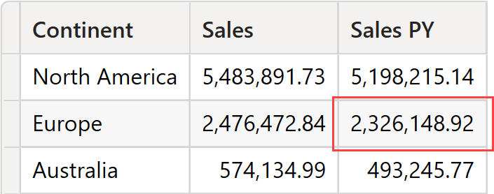
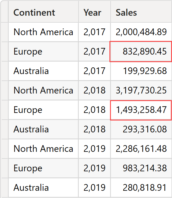
Let us focus on the highlighted cell for Europe. The filter context is defined by the current value of the continent (Europe) and the filter placed on the Date[Year] column, which is 2018 and 2019.

OFFSET generates the source table by grouping ALL ( Sales ) by Customer[Continent] and Date[Year]. Therefore, all the combinations of Continent and Year are present.

The source table contains multiple rows for Europe: one per year. In this scenario, defining the current row becomes trickier. Here is where the full “apply semantics” algorithm comes in handy. Let us describe the algorithm.

First, matching takes place. OFFSET analyzes the model columns in the source table and detects which columns are present in the evaluation context and their visible values.

• Customer[Continent] is in the filter context generated by SUMMARIZECOLUMNS. It shows only one value: Europe. Customer[Continent] is marked as a bound column.
• Date[Year] is present in the filter context, showing two values: 2018 and 2019. Date[Year] is marked as a bound column.

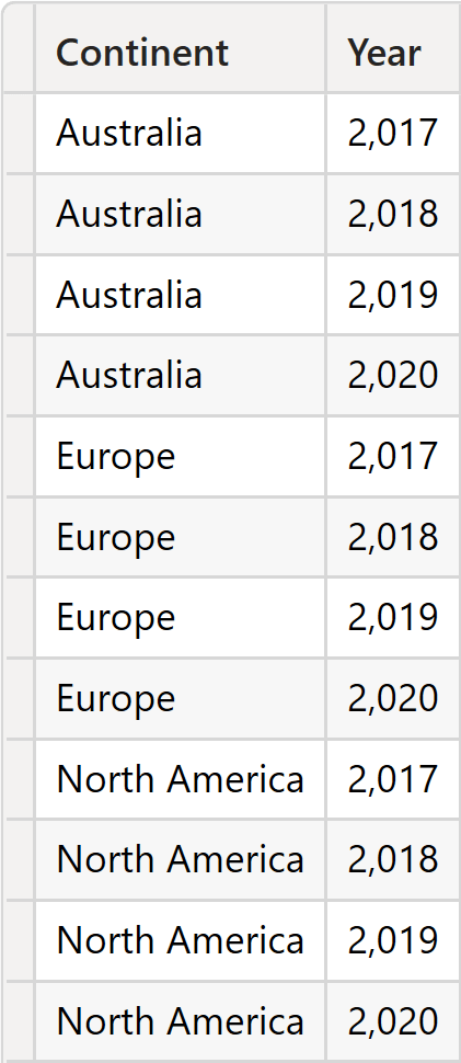
The matching table looks like this.

Continent	Year
Europe	2018
Europe	2019

OFFSET uses the matching table to filter the source table. Because all columns and values are present in the source table, the apply table is the same as the matching table. The matching table contains two rows: both are considered the current row.

OFFSET is now executed once per row in the matching table, generating the result.

Continent	Year
Europe	2017
Europe	2018

 

The result is thus Europe in 2017 and 2018. We can double-check the result by checking the sales by year and continent. The sum of the two highlighted cells produces the result of Europe in the previous DAX query: 2,326,148.92.

As you have seen in this example, using “apply semantics” makes it possible to obtain multiple current rows that correspond to multiple evaluations of OFFSET; using “apply semantics” makes it possible to obtain the correct result.

In most scenarios, developers do not need to understand all the details of “apply semantics”. A formula often performs an iteration over a table and computes OFFSET based on that same table. In this case, “apply semantics” produces only one row as its output. In more complex scenarios, like the ones we have shown so far with multiple results, OFFSET can produce multiple rows as its output.

Developers have the option of choosing which columns to consider in the “apply semantics” algorithm.

Apply semantics example (2)

Let us elaborate further on the “apply semantics” algorithm with another example. For each category, we want to find the previous one based on the sales amount sort order:

EVALUATE
VAR OriginalTable =
    ADDCOLUMNS (
        ALL ( 'Product'[Category] ),
        "Amount", [Sales Amount]
    )
VAR SourceTable =
    SELECTCOLUMNS (
        ALL ( 'Product'[Category] ),
        "PrevCategory", 'Product'[Category],
        "PrevAmount", [Sales Amount]
    )
RETURN
    GENERATEALL (
        OriginalTable,
        OFFSET (
            -1,
            SourceTable,
            ORDERBY ( [PrevAmount] )
        )
    )
ORDER BY [Amount]

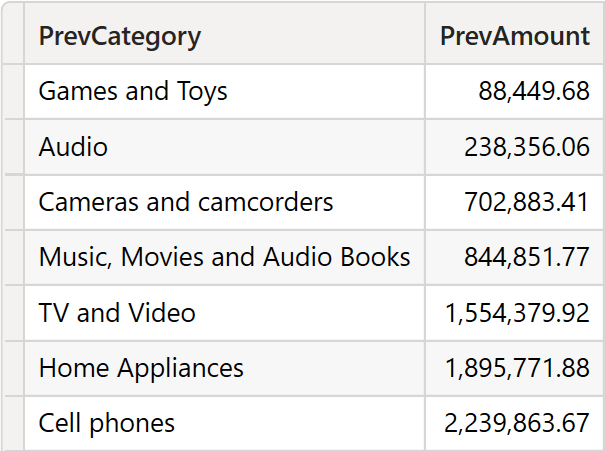
The result is a list containing one line for each category and amount, alongside the previous category and the corresponding amount.

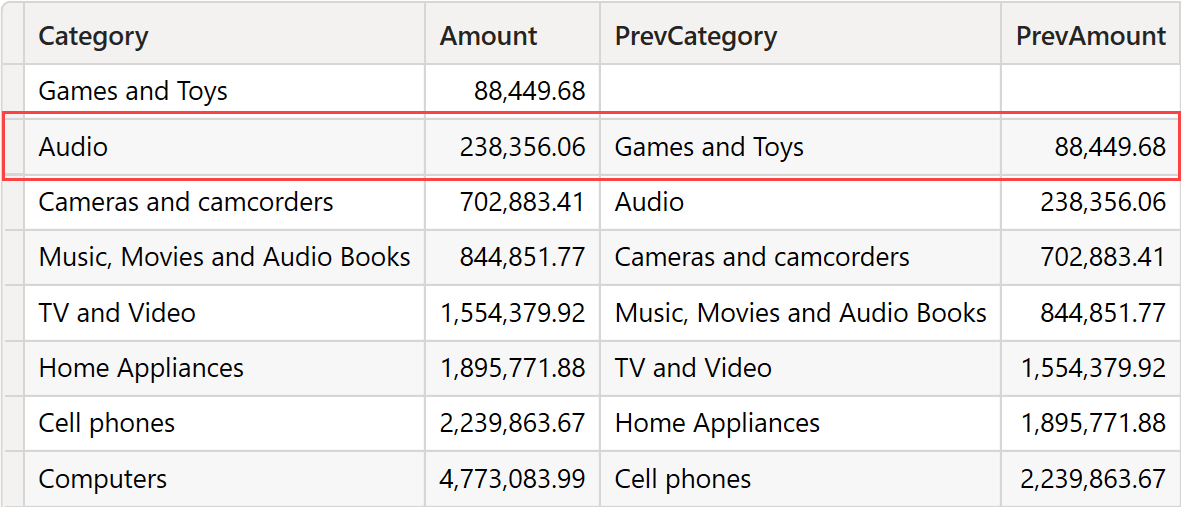
We are about to use the red boxed line in the following description. We are not interested in the result, but rather in the algorithm.

The source table contains two columns: PrevCategory and PrevAmount.

Despite its name, PrevCategory shares the data lineage of Product[Category]. Therefore, it is a model column. PrevAmount, on the other hand, is a local column created through a DAX function.

GENERATEALL iterates over OriginalTable, which contains Product[Category] and the Amount local column. Therefore, the row context includes both a model column (Product[Category]) and a local column (Amount). During the iteration, OFFSET is being executed. Let us pretend the iteration runs over the row (Audio, 238,356.06).

The only model column in the source table is matched with the current row context: Audio. As such, the matching table contains only one row with the value Audio. The matching table is used to filter the source table. Audio filters the PrevCategory column, and it finds the row (Audio, 238,356.06). Having reached this point, the engine found one current row. It executes OFFSET ( -1 ), thus finding (Games and Toys, 88,449.68). The result of OFFSET is joined with (Audio, 238,356.06), in turn producing the row we highlighted in the previous figure.

Let us analyze the same query, this time without GENERATEALL:

EVALUATE
VAR SourceTable =
    SELECTCOLUMNS (
        ALL ( 'Product'[Category] ),
        "PrevCategory", 'Product'[Category],
        "PrevAmount", [Sales Amount]
    )
RETURN
    OFFSET (
        -1,
        SourceTable,
        ORDERBY ( [PrevAmount] )
    )
ORDER BY [PrevAmount]

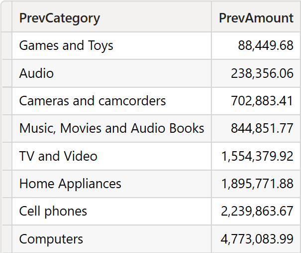
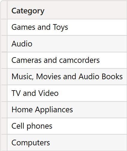
The beginning is identical. However, during the matching, there is no row context to provide a value for Product[Category]. Therefore, VALUES ( Product[Category] ) is evaluated in the current filter context, resulting in all the possible values of the Product[Category] column. This time, the matching table contains 8 rows: one per category.

Once the matching table filters the source table, the full source table is the current row. Therefore, OFFSET is executed 8 times, and the results are union-ed together. The first execution produces a blank result because there is no previous row. All remaining executions return the previous row. Therefore, the result contains all rows except the last one.

Conclusions

Apply semantics provides a result by finding the current row in scenarios where the very concept of current row is hard to define. Its behavior is totally intuitive in most cases, because when you use a window function, you likely build the query by providing the current row.

When the current row is not easily defined, apply semantics still works by creating a multi-row matching table and potentially a multi-row apply table. At this point, the results can be confusing. However, despite being confusing, they are legitimate, and they follow the precise algorithm of apply semantics.

Most developers will never have to deal with such complexity. However, mastering DAX requires a certain understanding of these complex aspects, so that we can always control the results of any measure.

Find more in the Understanding Visual Calculations in DAX whitepaper available to SQLBI+ subscribers