We dedicated a previous article to the blank row in DAX. In that article, the goal was to explain the differences between VALUES and DISTINCT. This article here focuses on how important it is to generate the blank row to guarantee that totals are always correct.
The blank row is created for regular relationships that are invalid – that is, when there is at least one row on the many-side that does not have a matching row on the one-side of the regular relationship. The same does not happen for limited relationships, which do not generate a blank row in similar conditions. Therefore, if a model contains a limited invalid relationship, developers must pay extra attention to how they create reports to avoid obtaining inaccurate results.
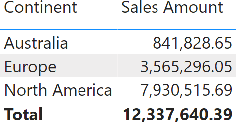
For example, look at the following report that contains only three rows.

Sales are sliced by continent; the total is the sum of individual rows. Right now, the relationship between Customer and Sales is valid, meaning that all the customer keys in Sales reference an existing row in Customer.
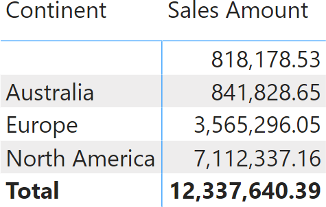
We make the relationship invalid by removing all the customers in California. Because the relationship is now invalid, DAX creates a blank row which is immediately visible in the report.

A total sales amount of 818,178.53 has been removed from North America (where California is) and is now visible in the blank row. The grand total is still the sum of individual rows. Therefore, the relationship is invalid, but the report works smoothly, clearly showing that a certain amount cannot be allocated to any continent.
In general, newbies dislike the blank row. It appears out of nowhere, and there are no ways to find it in the Power BI Desktop data view. Besides, it makes blanks appear in any slicer and report. However, the blank row exists for a very good reason: to ensure that the report shows correct values.
The blank row is not created if the relationship linking the two tables is limited. However, if the blank row is not part of the model, then a report cannot show the amount that is not related to a valid customer. Therefore, the net effect is that the individual rows still display their correct value; the total still shows the correct value, but the rows do not add up to the total because one row is missing: the blank row. Let us see this with an example.
A relationship is limited when it is either a cross-island relationship (for example, linking a table in DirectQuery mode with a table in VertiPaq mode) or a many-to-many cardinality relationship. For example, we can create a copy of the Customer table by using DirectQuery (Customer DQ). We remove California from the DirectQuery table, and finally we link Customer DQ to Sales.
The relationship between Customer DQ and Sales is limited because it crosses two islands. You can tell a relationship is limited because the edges of the relationship show a gap on both sides of the relationship.

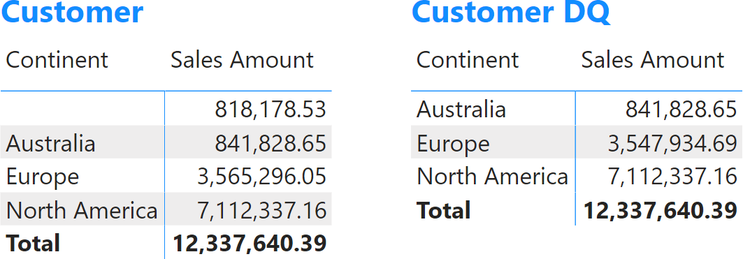
It is worth noting that the only difference between the two dimensions is the type of relationship that links them to Sales. What happens if we slice by the Continent column in Customer DQ rather than Customer? The following figure shows the two results side-by-side.

Individual continents show the same values, and so does the grand total. However, in the matrix slicing by Customer there is an additional row (the blank row) that accounts for the value missing to reach the total; that value is missing in Customer DQ.
From a user’s point of view, the visualization with the limited relationship (Customer DQ) is incorrect because the total value is different from the sum of the values for all continents. It is actually more wrong than the one showing the blank row (Customer). All the values are accounted for in the version with the blank row. The individual rows don’t sum up in the version without the blank row.
The same scenario occurs (albeit less frequently) if the relationship between two tables is set as a many-to-many cardinality relationship. The relationship is limited in that scenario as well, so the blank row is not enforced.
We imported Customer DQ as a VertiPaq table in the downloadable demo file and changed the relationship to a many-to-many cardinality. We obtained the same effect without using DirectQuery, which would not work on our readers’ computers as the Contoso database is stored on our servers.
Conclusions
The presence of a blank row in a table is a clear symptom of bad data. The blank row brings many calculation issues and is annoying because it shows blanks in all the slicers and tables browsed by users. Nonetheless, its existence is paramount to guarantee an accurate presentation of all the available data.
The correct way to handle the presence of a blank row is to clean your data, ensuring that all the relationships stand right. If the blank row is not enforced by DAX because you have limited relationships, then the numbers are no longer accurate.
In short: clean up your data, and the blank row will never bother you.
When a column name is given, returns a single-column table of unique values. When a table name is given, returns a table with the same columns and all the rows of the table (including duplicates) with the additional blank row caused by an invalid relationship if present.
VALUES ( <TableNameOrColumnName> )
Returns a one column table that contains the distinct (unique) values in a column, for a column argument. Or multiple columns with distinct (unique) combination of values, for a table expression argument.
DISTINCT ( <ColumnNameOrTableExpr> )
 Marco Russo & Alberto Ferrari