2023-03-05: one performance example in this article is no longer faster than the original version. As you can read in the comments, tests made in February 2023 demonstrate that the original version of a measure in this article performs now better than any of the other optimizations. This article is still good at showing how the data lineage works. However, the specific example showing a performance improvement is no longer valid. As usual, when you apply an optimization that makes the code more complex, you must be aware that you stop future versions of the engine from finding a better execution path for the simpler code. The technique shown in this article could still be valid in other scenarios, but it’s not an optimization for the sample used in the article.
Introducing data lineage
First things first, what is data lineage? Data lineage is a tag. Assigned to every column in a table, this tag identifies the original column in the data model that the values of a column originated from. For example, the following query returns the different categories in the Product table:
EVALUATE VALUES ( 'Product'[Category] ) |
The result contains 8 rows, one for each category:
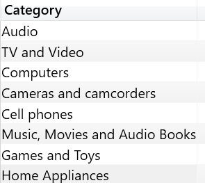
The table returned by VALUES contains 8 strings. Nevertheless, they are not just strings. DAX knows that these strings originated from the Product[Category] column. Therefore, being columns of the Product table, they inherit the capability of filtering other tables in the model following the filter propagation through relationships. This is the reason why a context transition iterating VALUES ( Product[Category] ) filters the Sales table. Consider the following query:
1 2 3 4 5 | EVALUATEADDCOLUMNS ( VALUES ( 'Product'[Category] ), "Amt", [Sales Amount]) |
The result of the query includes the value of Sales Amount for each product category:
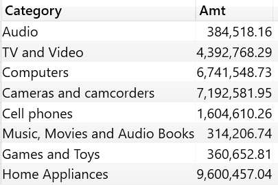
The string “Audio”, by itself, cannot filter Sales. You can easily check this by running the following query:
1 2 3 4 5 6 7 8 9 10 11 12 13 14 15 16 17 18 | EVALUATEVAR Categories = DATATABLE ( "Category", STRING, { { "Category" }, { "Audio" }, { "TV and Video" }, { "Computers" }, { "Cameras and camcorders" }, { "Cell phones" }, { "Music, Movies and Audio Books" }, { "Games and Toys" }, { "Home Appliances" } } )RETURN ADDCOLUMNS ( Categories, "Amt", [Sales Amount] ) |
The query returns the same value in the Amt column for all the rows:
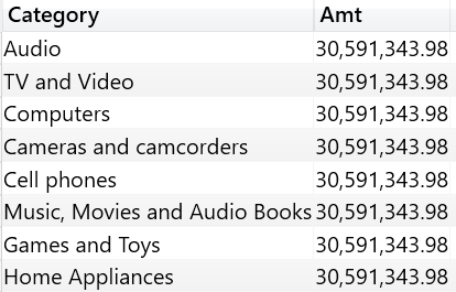
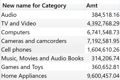
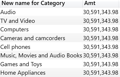
Neither the column name nor the column content are important. What really matters is only the data lineage of a column, which is the original column the values have been retrieved from. If a column is renamed, the data lineage is still maintained. Indeed, the following query returns a different value for every row:
1 2 3 4 5 6 7 8 | EVALUATEADDCOLUMNS ( SELECTCOLUMNS ( VALUES ( 'Product'[Category] ), "New name for Category", 'Product'[Category] ), "Amt", [Sales Amount]) |
The “New name for Category” column maintains the data lineage of Product[Category]. Therefore, the output shows the sales sliced by category, although the column name in the result is different from the original column name.
Data lineage is maintained as long as an expression is only made up of one column reference. For example, adding an empty string to Product[Category] in the previous expression does not change the column content, whereas it does break the data lineage. In the following code, the source of New name for Category is an expression instead of only being a column reference. As a result, the new data lineage of the new column is not related to any of the source columns of the model.
1 2 3 4 5 6 7 8 | EVALUATEADDCOLUMNS ( SELECTCOLUMNS ( VALUES ( 'Product'[Category] ), "New name for Category", 'Product'[Category] & "" ), "Amt", [Sales Amount]) |
Unsurprisingly, the result shows the same Amt value for all the rows.
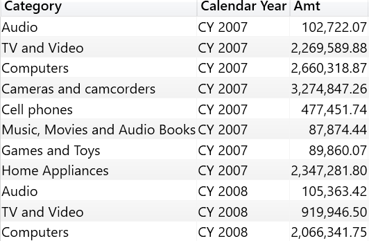
Each column has its own data lineage, even though a table contains columns originating from different tables. Therefore, the result of a table expression can apply filters to multiple tables at once. This is clearly visible in the following query, which contains both Product[Category] and Date[Calendar Year]. Both columns apply their filter to the Sales Amount measure through the filter context originated by context transition.
1 2 3 4 5 6 7 8 9 10 11 | EVALUATEFILTER ( ADDCOLUMNS ( CROSSJOIN ( VALUES ( 'Product'[Category] ), VALUES ( 'Date'[Calendar Year] ) ), "Amt", [Sales Amount] ), [Amt] > 0) |
The result shows the sales amount for the given category and year. Both the Category and Calendar Year columns are actively filtering the Sales Amount measure.
Even though the data lineage is kept and maintained by the engine in a completely automatic way, the developer has the option of changing the data lineage of a table. This is what the TREATAS function is useful for. TREATAS accepts a table as its first argument, followed by a list of column references. TREATAS returns the same input table, with each column tagged with the data lineage of the column references specified as arguments. If some of the values in the table contain values that do not correspond to a valid value in the column used to apply the data lineage change, then TREATAS removes the values from the input. For example, the following query builds a table with a list of strings, one of which (the highlighted one, “Computers and geeky stuff”) does not correspond to any category in the model. We used TREATAS to force the data lineage of the table to Product[Category].
1 2 3 4 5 6 7 8 9 10 11 12 13 14 15 16 17 18 19 20 21 22 23 24 | EVALUATEVAR Categories = DATATABLE ( "Category", STRING, { { "Category" }, { "Audio" }, { "TV and Video" }, { "Computers and geeky stuff" }, { "Cameras and camcorders" }, { "Cell phones" }, { "Music, Movies and Audio Books" }, { "Games and Toys" }, { "Home Appliances" } } )RETURN ADDCOLUMNS ( TREATAS ( Categories, 'Product'[Category] ), "Amt", [Sales Amount] ) |
The result contains sales sliced by category, but the row containing Computers and geeky stuff is missing from the output.
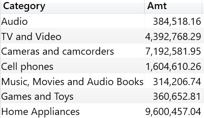
In the data model there is no category named “Computers and geeky stuff”, therefore TREATAS had to remove the row from the output in order to complete the data lineage transformation.
Manipulating data lineage
Now that we have seen what data lineage is and how to manipulate it by using TREATAS, it is time to see an example where TREATAS and data lineage manipulation produce very elegant DAX code. Consider the requirement of computing the Sales Amount, filtering only the first day of sales for each product. The same calculation can be meaningful by customer, by store, or by any other dimension, yet we only consider the products in this example.
Each product has a different first-sale date. One option is to compute the first date of sales iterating on a product-by-product basis, then compute the Sales Amount in that date and finally aggregate the results for all the products. The following code works just fine:
1 2 3 4 5 6 7 8 9 10 11 12 13 | FirstDaySales v1 :=SUMX ( 'Product', VAR FirstSale = CALCULATE ( MIN ( Sales[Order Date] ) ) RETURN CALCULATE ( [Sales Amount], 'Date'[Date] = FirstSale )) |
The result produced by the FirstDaySales measure shows a subset of Sales Amount for each Brand.
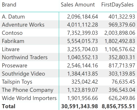
The result is correct, but the code above is not optimal. Indeed, it iterates the Product table generating a context transition for each product, also applying a filter on Date without leveraging any relationship. Not to say that this is bad code, it is just not as elegant as it could be. We will now see alternative versions of this measure return the same result in a more efficient manner.
A first step in the right direction is to build a table containing the product name and the corresponding date of the first sale, then use this pair to apply a filter on Sales. The following code is an improvement compared to the previous code, but it is still non-optimal because SUMX still generates a context transition for each product:
1 2 3 4 5 6 7 8 9 10 11 12 13 14 15 16 17 18 19 20 21 22 23 | FirstDaySales v2 :=VAR ProductsWithSales = SUMMARIZE ( Sales, 'Product'[Product Name] )VAR ProductsAndFirstDate = ADDCOLUMNS ( ProductsWithSales, "Date First Sale", CALCULATE ( MIN ( Sales[Order Date] ) ) )VAR Result = SUMX ( ProductsAndFirstDate, VAR DateFirstSale = [Date First Sale] RETURN CALCULATE ( [Sales Amount], 'Date'[Date] = DateFirstSale ) )RETURN Result |
However, focus your attention on the result of ADDCOLUMNS in the ProductsAndFirstDate variable. It contains a product name and a date. If used as a filter argument of CALCULATE, it will filter a product and a date. Therefore, this version (which is wrong, unfortunately) would be better:
1 2 3 4 5 6 7 8 9 10 11 12 13 14 15 16 17 18 19 | FirstDaySales v3 (wrong) :=VAR ProductsWithSales = SUMMARIZE ( Sales, 'Product'[Product Name] )VAR ProductsAndFirstDate = ADDCOLUMNS ( ProductsWithSales, "Date First Sale", CALCULATE ( MIN ( Sales[Order Date] ) ) )VAR Result = CALCULATE ( [Sales Amount], ProductsAndFirstDate )RETURN Result |
As you see, the SUMX iteration disappeared from the algorithm. Nevertheless, this version of the code is flawed, because it returns the same value as Sales Amount without applying any filter. Indeed, the result of ADDCOLUMNS in ProductsAndFirstDate contains a product and a date; but from a data lineage point of view the product name is of type Product[Product Name] whereas the date in the First Sale column does not have the data lineage of date, being the result of a MIN expression. The First Sale column has its own data lineage, which is unrelated to the other tables in the data model.
The solution is to change the data lineage of the First Sale column to force it to be Date[Date]. TREATAS exists for this precise purpose. The correct optimized measure is the following:
1 2 3 4 5 6 7 8 9 10 11 12 13 14 15 16 17 18 19 20 21 22 23 24 25 | FirstDaySales v4 :=VAR ProductsWithSales = SUMMARIZE ( Sales, 'Product'[Product Name] )VAR ProductsAndFirstDate = ADDCOLUMNS ( ProductsWithSales, "First Sale", CALCULATE ( MIN ( Sales[Order Date] ) ) )VAR ProductsAndFirstDateWithCorrectLineage = TREATAS ( ProductsAndFirstDate, 'Product'[Product Name], 'Date'[Date] )VAR Result = CALCULATE ( [Sales Amount], ProductsAndFirstDateWithCorrectLineage )RETURN Result |
Solutions like this last one do not come to mind as a primary solution to the pattern. Nevertheless, performance-wise this code is nearly optimal, which means that we did not find a better performing version – if you do find a better one, we would love to see it in the comments. You will start thinking of solutions like the one above once you are acquainted with data lineage, understanding how the filter moves from one table to another by using data lineage.
Conclusions
In the DAX developer’s tool belt, understanding data lineage is one important skill. It is not as primordial as row context, filter context and context transition are. Yet, it is for sure one of the skills that distinguish professional DAX developers from the rest.
When a column name is given, returns a single-column table of unique values. When a table name is given, returns a table with the same columns and all the rows of the table (including duplicates) with the additional blank row caused by an invalid relationship if present.
VALUES ( <TableNameOrColumnName> )
Treats the columns of the input table as columns from other tables. For each column, filters out any values that are not present in its respective output column.
TREATAS ( <Expression>, <ColumnName> [, <ColumnName> [, … ] ] )
Returns the sum of an expression evaluated for each row in a table.
SUMX ( <Table>, <Expression> )
Returns a table with new columns specified by the DAX expressions.
ADDCOLUMNS ( <Table>, <Name>, <Expression> [, <Name>, <Expression> [, … ] ] )
Evaluates an expression in a context modified by filters.
CALCULATE ( <Expression> [, <Filter> [, <Filter> [, … ] ] ] )
Returns the smallest value in a column, or the smaller value between two scalar expressions. Ignores logical values. Strings are compared according to alphabetical order.
MIN ( <ColumnNameOrScalar1> [, <Scalar2>] )
 Alberto Ferrari
 Copy
Copy Conventions