Banding with PowerPivot

Banding is one of the most common requirements when you have the need to analyze continuous values, like the retail price of a product which may change over time, due to discounts and price variations. I have already spoken about banding with regards to SSAS here, now I would like to spend some words on banding with PowerPivot. This topic is covered in much more details in the upcoming book I have written with Marco Russo: “Microsoft PowerPivot for Excel 2010: Give Your Data Meaning”.

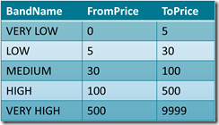
To show the examples, I am using the fact reseller sales table in AdventureWorks and this banding table:

Now, let us take a look at the various options that we have available in PowerPivot to perform banding.

The first one is the naïf one. You can add a calculated column with a long formula that computes the price band:

= IF (     FactResellerSales[DiscountedPrice] <= 5,     "01 LOW",      IF (         FactResellerSales[DiscountedPrice] <=30,          "02 MEDIUM",         IF (             FactResellerSales[DiscountedPrice] <=100,              "03 MEDIUM",              IF (                 FactResellerSales[DiscountedPrice] <= 500,                  "04 HIGH",                  "05 VERY HIGH"))))

It is quick, dirty, but it works. Clearly, even if I expect that this approach will be used by many Excel users, I don’t think that this formula is worth a post . Moreover, using this approach requires you to update the formula whenever you want to change the banding table (which is hardcoded inside the formula) thus, in the search for a better data driven approach, I am going to show some better solutions.

Nevertheless, even if I don’t like this formula, it is worth noting that with PowerPivot you have a quick and dirty option. If you (as I do) extensively use PowerPivot to perform fast prototyping of complex BI solutions, then you will be able to show banding to end users with a real minimal effort. Then, when the demo is finished, it is time to search for something better.

A second approach would be that of relying on the PowerPivot engine to create a relationship between the FactResellerSales table and the band one. Nevertheless, you cannot create such a relationship since the banding table, in its current format, does not have a valid key. It contains ranges, not values which can be the target of a relationship. Nevertheless, performing a simple change in the data model, you can follow the same approach used with SSAS and expand the banding table so that it gains a structure which can be used to create the relationship.

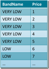
The new band table format might be like this:

Now, Price is a valid key and you can create a relationship between the FactResellerSales table and this table using the price. Clearly, since this table is too long to be filled by hand, you will need to create a simple VBA script that starts from the previous table and creates the expanded one, where each band is repeated for each single price. The code is not complex and might look like this:

For Each Row In ActiveSheet.ListObjects("PriceBands").ListRows     Dim MinValue As Integer     Dim MaxValue As Integer     Dim Value As Integer     Dim newRow As ListRow     MinValue = Row.Range(1, 2).Value     MaxValue = Row.Range(1, 3).Value - 1     For Value = MinValue To MaxValue         Set newRow = PriceBandsExpanded.ListRows.Add         newRow.Range(1, 1) = Row.Range(1, 1)         newRow.Range(1, 2) = Value      Next Next 

This solution works in a data driven way, is very simple to implement and solves the banding problem. Nevertheless, it requires one step (the creation of the expanded table) every time you update the configuration sheet. Moreover, it requires a bit of knowledge of VBA programming, which might not be in the hands on the average Excel user. Thus, it is better to find a pure PowerPivot solution to banding.

The key point here is that we want to create a relationship based on BETWEEN, while in PowerPivot we can only leverage relationships based on identity of values. Thus, to override the limitation of PowerPivot, it will be necessary to avoid using its engine and leverage the full power of DAX to create a calculated column that mimics the BETWEEN relationship.

Let us revert back to our original table, let us suppose that we create a linked table inside PowerPivot and call it PriceBands. We do not create any relationship between FactResellerSales and PriceBands, instead we can leverage the FILTER function to find, for each row of the sales, the correct price band. My first trial has been this:

BandName=MAXX (     FILTER (         PriceBands,         FactResellerSales[DiscountedPrice] >= PriceBands[MinPrice]       && FactResellerSales[DiscountedPrice] < PriceBands[MaxPrice]     ),    [PriceBand] )

In this formula we leverage FILTER to fine the PriceBands table and find the right row. Now, since FILTER returns a table (which, we know, contains only one row), we use MAXX to transform this table into a scalar value, which should contain the PriceBand name. As simple as this solution seems, it will not work because the MAXX function in PowerPivot does not work with strings, it only computes MAX of numbers or dates. If you wonder why, as I do, you’d better know that this is for “Excel compatibility”, thus it is by (wrong) design. The very creative reader might now think at a new solution, that is add an identity column to the PriceBand table, compute the MAX of that identity value (which is now a number, thus MAXX will work) and then use it to setup a relationship with the PriceBand table. Believe me, it will work fine (I tested it) but, clearly, it is not very elegant.

The elegant solution is to leverage the CALCULATE function. By using CALCULATE you will end up with this formula:

BandName = CALCULATE(     VALUES (PriceBands[PriceBand]),     FILTER (         PriceBands,          FactResellerSales[DiscountedPrice] >= PriceBands[MinPrice]      && FactResellerSales[DiscountedPrice] < PriceBands[MaxPrice]     ) )

The key is to use CALCULATE to create a new execution context where the PriceBand table is filtered so that it will contain only one row, using the same filter expression used before. Then, when PowerPivot calculates the VALUES (PriceBands[PriceBand]) expression to compute the distinct values of the PriceBand column, it performs the calculation in a context where there exists only one row, so the returning value will be the right band name. If, for some error in the configuration, the VALUES call returns more than one row, PowerPivot will raise an error. Otherwise, it the resulting table contains one row only, then the value is automatically converted into a scalar value and the formula correctly computes the band name.

As it often happens with PowerPivot, the correct solution requires you to use and understand CALCULATE, and to have a creative mind to search for non trivial solutions to the problem. Nevertheless, the final result is a very compact, elegant and fast formula that works in a complete data drive way and let the user change the configuration sheet, refresh data and test several bandings at a glance.

.csharpcode, .csharpcode pre { font-size: small; color: black; font-family: consolas, “Courier New”, courier, monospace; background-color: #ffffff; /*white-space: pre;*/ } .csharpcode pre { margin: 0em; } .csharpcode .rem { color: #008000; } .csharpcode .kwrd { color: #0000ff; } .csharpcode .str { color: #006080; } .csharpcode .op { color: #0000c0; } .csharpcode .preproc { color: #cc6633; } .csharpcode .asp { background-color: #ffff00; } .csharpcode .html { color: #800000; } .csharpcode .attr { color: #ff0000; } .csharpcode .alt { background-color: #f4f4f4; width: 100%; margin: 0em; } .csharpcode .lnum { color: #606060; }