Dynamic Ranking with Excel and PowerPivot

Ranking is useful and, in our book, I and Marco provide a lot of information about how to perform ranking with PowerPivot. Nevertheless, there is an interesting scenario where ranking can be performed without complex DAX formulas, but with just some creative Excel usage. I would like to describe it here.

Let us start with some words about the scenario: we want to rank products based on sales in a year (e.g. 2002) and see how the top 10 of these products performed in the following or preceding years.

Let us start loading inside PowerPivot some tables from the AdventureWorksDW database: DimProduct, FactInternetSales and DimTime. We can then use a PivotTable to see sales in 2002 (using the slicer) and, leveraging the sorting option of the PivotTable, we sort by SalesAmount, putting the best performers on top.

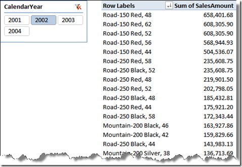
Doing this, we have solved the first part of the scenario, i.e. we have identified which are the best products in 2002, yet what we want to do is to perform an analysis on how they performed during subsequent years. To do so, we must first assign a ranking number and/or category to each product, and then reload this table inside PowerPivot, so that we can use the ranking category as a new slicer in a new PivotTable.

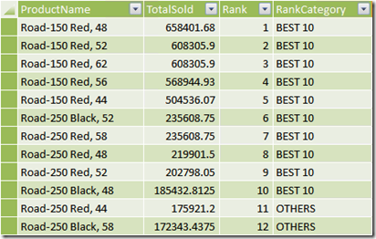
There is no way to reload the result of a PivotTable inside PowerPivot directly. Nevertheless, by simply copying the result of the PivotTable inside an Excel Range, we can then format that range as a table and link it into Excel. In the following picture I did exactly this, using very simple Excel formulas to compute the rank (i.e. ROW() – 4) and the RankCategory (if rank is less than 10, then “BEST 10” else “OTHERS”):

Now, before we format the range as a table, we need to face a small issue: if we later decide to change the slicer to 2001 or to change in any way the filters, the number of products returned by the PivotTable will change, resulting in less or more rows, depending on the filter. Since we want to assign a rank to ALL of the products, we want the PivotTable to always return all the products, regardless of the filter. This can be easily accomplished using the PivotTable Options of Excel, asking to show even rows with no data:

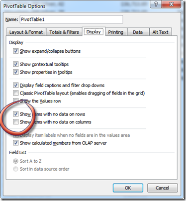
Now, the PivotTable will always return all the products. We can complete our Excel range with the correct formulas, format is as a table and call it RankedProducts. Done it, we can use the Linked Table feature of PowerPivot and load it inside the Vertipaq engine:

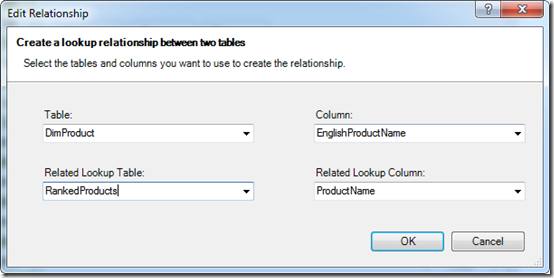
The work is almost done. We still need to create a relationship between RankedProducts and DimProduct, as shown in the next figure:

Now everything is ready for our report: just create a new PivotTable, put the RankCategory on the slicer, the product name on rows, the year on columns and SalesAmount on values, the resulting report satisfies our initial request: products are filtered based on the ranking in 2002 but the values shown are pertinent to all the years available in the database:

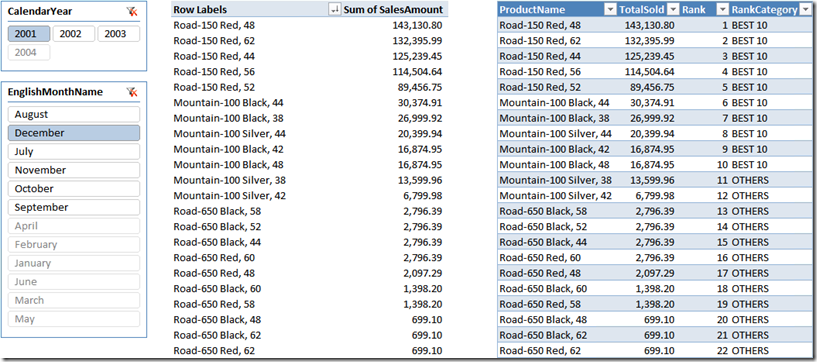
The interesting part of this scenario is that now, if we want to change the ranking filter using a different selection for time (in the following example we have ranked based on December 2001), it is enough to use the Update All button in the PowerPivot tab of the Ribbon to reload the new RankedProducts table and get a complete different ranking. The very same technique can be used to create custom sets and many other interesting analysis, which is something I leave to your imagination.

As you can see, all of this has been done without ever writing a single line of DAX. Does it mean that DAX is not useful? Not at all, using DAX we can get much more powerful reports, nevertheless this is some kind of real self service BI, that can be authored by an Excel Power User with some basic knowledge of PowerPivot and a creative mind.

This is just a very simple example of what PowerPivot can do for your reporting needs. If you want to touch the real Karma of PowerPivot, don’t miss the opportunity to follow one of the workshops I and Marco Russo are bringing all over Europe in the next few months.

You can find more info on www.powerpivotworkshop.com. Hope to see you  there!