PowerPivot, Stocks Exchange and the Moving Average

In this post I want to analyze a data model that perform some basic computations over stocks and uses one of the most commonly needed formula there (and in many other business scenarios): a moving average over a specified period in time. Moving averages can be very easily modeled in PowerPivot, but there is the need for some care and, in this post, I try to provide a solid background on how to compute moving averages.

In general, a moving average over period T1..T2 is the average of all the values between T1 and T2. Sounds easy, so why do I feel the need to write a post about it? Because in stock fixings, as in sales and many many other scenarios, the moving average cannot be computed that easily. If the period is – say – 10 days, then it can contain one or more holidays inside. during holidays, there is no data and this does not mean that the value during holidays does not exists, it means that holidays should not be used to compute the average. Moreover, different periods contain a different number of vacation days, making things a little bit more complicated.

The business scenario is clear, let us describe the data model. We basically have one table, called Fixing, which contains the value of stocks for the last 10 years:

There are a lot of columns here, since this is the data structure provided by my trading system but we are interested in only three columns, for the sake of this example:

• Stock: the name of the stock, i.e. Microsoft.
• Date: the date of the values
• Close: the final price of the stock

As a very gross rule of thumb, if the price of the stock is higher than the moving average over a period of time, then the price of the stock will further increase, if it is below the moving average, it will decrease further. Normally two moving averages are used in conjunction and the points where the stock is changing direction are detected by the intersection of the two moving averages.

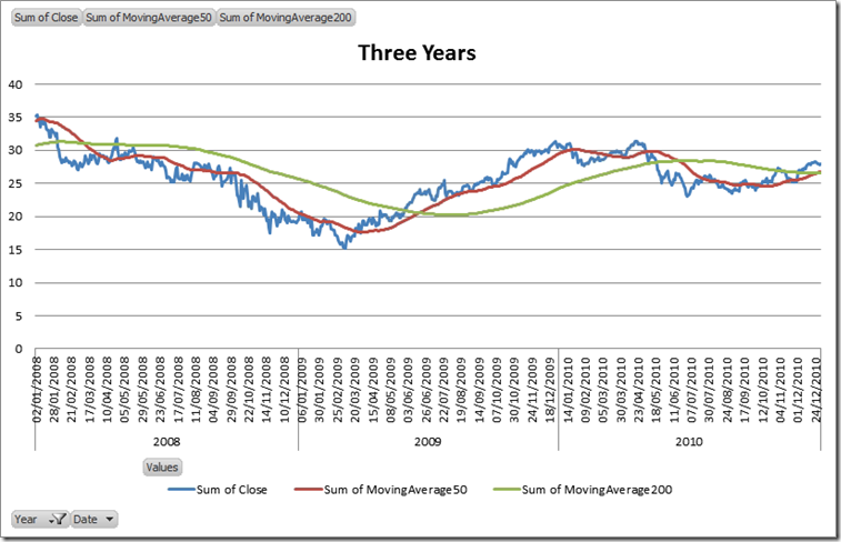
Thus, we want to use PowerPivot to produce a chart like the following one, which represents the last three years of the Microsoft stock. When the red line crosses the green one going down, it is time to sell, when it crosses going up it is time to buy. If you use this rule to trade… don’t blame me for any loss, I only tried to explain why moving averages are pretty useful in the stocks market.

Now, let us get back to business: how do we compute the moving average? In a previous post, I spoke about how to compute the difference in working days between two dates. This scenario is very similar since the moving average over 50 days is, in fact, the average of the last 50 “working” days of the trading market, i.e. the dates where the value of the stock exists in our table. Thus, the problem is now shifted to “how do I compute the date that is 50 working days before the current one?”.

The answer is pretty easy: first of all we need to assign to each date in the tale an incremental number, counting the number of dates before the current one. Clearly, since we have many different stocks in the table, we must count only the dates where the price of the current stock exists. Let us add a calculated column to the Fixing table with this formula:

DayNumber =
COUNTROWS (
    FILTER (
        Fixing,
        Fixing[Date] <= EARLIER ( Fixing[Date] )
            && Fixing[Stock] = EARLIER ( Fixing[Stock] )
    )
)

Now each row in the Fixing table has a number that uniquely identifies each date for a stock. Let us add a new calculated column to hold the date that represents “50 working days before now”:

FirstDateOfRange50 =
CALCULATE (
    VALUES ( Fixing[Date] ),
    FILTER (
        Fixing,
        Fixing[DayNumber] = EARLIER ( Fixing[DayNumber] ) - 50
            && Fixing[Stock] = EARLIER ( Fixing[Stock] )
    )
)

Basically, we use CALCULATE to get VALUES of the Date column in a filter context that shows the only one row that has a DayNumber equals to the current day number less 50. Now that we have the value of the first date of the range, knowing that the last date of the range is always the current date, we can compute the moving average over 50 days using this formula:

=
CALCULATE (
    AVERAGE ( Fixing[Close] ),
    FILTER (
        Fixing,
        Fixing[Date] >= EARLIER ( Fixing[FirstDateOfRange50] )
            && Fixing[Date] <= EARLIER ( Fixing[Date] )
            && Fixing[Stock] = EARLIER ( Fixing[Stock] )
    )
)

The key here is the FILTER expression, that creates a filter context that shows 50 rows from the Fixing table, exactly the 50 rows that are needed to compute our moving average. Repeating the same procedure for the 200 days average, you end up with this table inside PowerPivot:

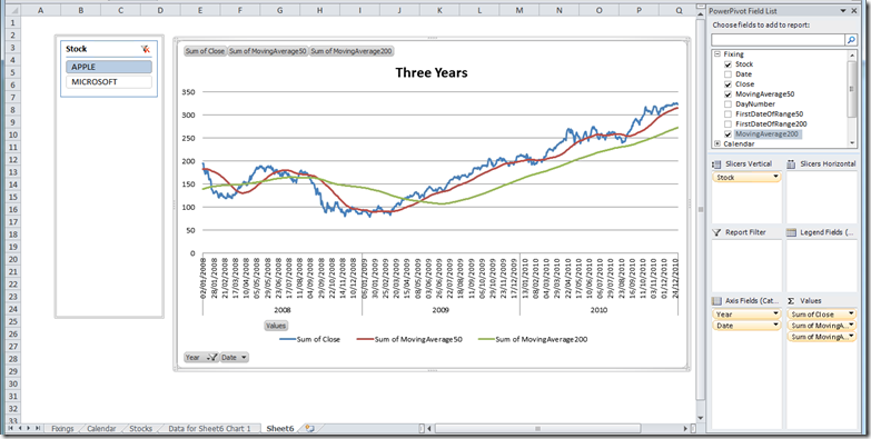
Et voilà, the hard part of the work is done. The remaining work is just to add a PivotChart as in the following figure. where we have selected Apple instead of Microsoft:

As you can see from the figure, I added the Calendar table to the data model with the necessary relationship to be able to add the year to the chart but, this time, I did not use the Calendar table to perform working days computation since the addition of the stock name makes the model a bit more complex (a date might be “working” for a stock but not for another one) and the DAX formulas need to be more complex too.

This is just another example of what PowerPivot can do for your reporting needs. If you want to touch the real Karma of PowerPivot, don’t miss the opportunity to follow one of the workshops I and Marco Russo are bringing all over Europe in the next few months.

You can find more info on www.powerpivotworkshop.com. Hope to see you  there!