PowerPivot and Parent/Child hierarchies

Does PowerPivot handle Parent/Child hierarchies? The common answer is “no”, since it does not handle them natively. During last PowerPivot course in London, I have been asked the same question once more and had an interesting discussion about this severe limitation of the PowerPivot data modeling and visualization capabilities. On my way back in Italy, I started thinking at a possible solution and, after some work, I managed to make PowerPivot handle Parent/Child hierarchies in a very nice way, which is indistinguishable from SSAS. This post explains the technique.

Before starting the real topic of the post, I need to say a couple things:

1. This is definitely NOT self service BI. I am going to adopt advanced data modeling techniques and, to fully understand how the formulas work, you need to have a good understanding of the DAX behavior in terms of filter contexts. From the SQL point of view, on the other hand, only a basic understanding of CTE is required.
2. After one day of hard work on this topic, my desktop was loaded with sheets of papers full of doodles and the test workbook contained an insane number of non-working formulas. It has been a phone call with Marco Russo which really turned on the light into the solution, we definitely work fine as a team! Thus, I share the merit of the post with Marco, and I feel the need to make it clear.

And now, let’s get back to business, and start the topic.

Let us suppose that we have a hierarchy of sales persons, like this:

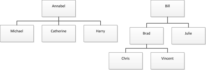
This hierarchy has two root nodes and then some children, with a maximum depth of three levels. Each individual in this chart produces sales, stored in an invoice table that contains a reference to the individual. Data is stored in the classical way inside two tables: Tree contains the hierarchy and Invoices contains the invoices. The table structure is the following:

CREATE TABLE Tree (     NodeID INT,     Node VARCHAR (100),     ParentID INT)  CREATE TABLE Invoices (     NodeID INT,      InvoiceID INT,      Amount INT,      City VARCHAR (100) )

Once you have created the tables, you can populate them with sample data using this script, that creates the hierarchy and puts some values in the invoices:

INSERT INTO Tree VALUES  ( 1, 'Bill',       NULL),         ( 2, 'Brad',       1),         ( 3, 'Julie',      1),         ( 4, 'Chris',      2),         ( 5, 'Vincent',    2),         ( 6, 'Annabel',    NULL),         ( 7, 'Catherine',  6),         ( 8, 'Harry',      6),         ( 9, 'Michael',    6);  INSERT INTO Invoices VALUES (2,  3, 200, 'Chicago'),        (2,  4, 200, 'Seattle'),        (3,  5, 300, 'Chicago'),        (4,  6, 400, 'Seattle'),        (5,  7, 500, 'Chicago'),        (6,  8, 600, 'Seattle'),        (7,  9, 600, 'Seattle'),        (7, 10, 600, 'Chicago'),        (8, 11, 400, 'Chicago'),        (8, 12, 400, 'Seattle'),        (9, 13, 300, 'Chicago'),        (9, 14, 300, 'Seattle');

Before explaining the technique, let us take a look at the final result. We want to obtain this PivotTable:

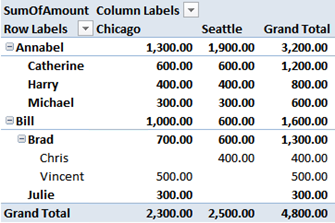
The notable aspects to look at are only two:

• There are three levels in the hierarchy but, since the first tree, starting with Annabel, has a maximum depth of two, we don’t want to see the third level, which does not contain useful information.
• The total of each node is the sum of all of its children plus the value produced by the node itself. If you look, for example, at the value of Brad in Chicago, it is 700.00, even if Vincent has produced 500,00. This means that 200,00 has been produced by Brad.

We are going to reach the final result step by step, starting from a very basic visualization and then solving the various issues, as they will become evident.

If we load the two tables inside PowerPivot, setup the relationships and create a PivotTable, we will end up with this:

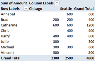
The totals are correct, but don’t take into account the hierarchy, they represent only the total sales of each individual. Said in other words, PowerPivot has no knowledge at all of the existence of the self-relationship and behaves in a classical way, aggregating values by node. In order to create a hierarchy, we will need to add columns to the tree table that let us slice data following the Parent/Child hierarchy. There is a well-known technique to use, which is called “Naturalized Parent/Child” and that requires to:

• Define the maximum depth of the hierarchy. Since in our case we have three levels at maximum depth, we can start with a hierarchy with some free space, let us say that five levels are good.
• Create a column for each level which contains the parent of the node at that level.

Since this is a classical technique, I am not going to explain it in full detail. The result can be obtained with a SQL query that implements recursive CTE like this:

DECLARE @KeyLength INT = 3;  WITH      FindNodePaths AS (         SELECT              NodeId    = NodeID,              NodePath  = CAST (' '                                + RIGHT (REPLICATE ('0', @KeyLength)                                + CAST (NodeID AS VARCHAR (100)), @KeyLength) AS VARCHAR (100))         FROM Tree WHERE ParentID IS NULL         UNION ALL         SELECT              NodeId    = Tree.NodeID,              NodePath  = CAST (NodePath + ' '                                + RIGHT (REPLICATE ('0', @KeyLength)                                + CAST (Tree.NodeID AS VARCHAR), @KeyLength) AS VARCHAR (100))         FROM Tree             INNER JOIN FindNodePaths AS Parent ON Parent.NodeID = Tree.ParentID     ),     ComputeParentNodeIdAtLevels AS (         SELECT              NodeID                = NodeID,             NodePath              = NodePath,             ParentNodeIdAtLevel1  = SUBSTRING (NodePath, 2, @KeyLength),             ParentNodeIdAtLevel2  = SUBSTRING (NodePath, (@KeyLength + 1) * 1 + 2, @KeyLength),             ParentNodeIdAtLevel3  = SUBSTRING (NodePath, (@KeyLength + 1) * 2 + 2, @KeyLength),             ParentNodeIdAtLevel4  = SUBSTRING (NodePath, (@KeyLength + 1) * 3 + 2, @KeyLength),             ParentNodeIdAtLevel5  = SUBSTRING (NodePath, (@KeyLength + 1) * 4 + 2, @KeyLength)         FROM FindNodePaths     ) SELECT      NodeId   = C.NodeId,     Node     = T.Node,     Level1   = T1.Node,     Level2   = T2.Node,     Level3   = T3.Node,     Level4   = T4.Node,     Level5   = T5.Node FROM      ComputeParentNodeIdAtLevels C         LEFT OUTER JOIN Tree T  ON T.NodeID = C.NodeID         LEFT OUTER JOIN Tree T1 ON T1.NodeID = C.ParentNodeIdAtLevel1         LEFT OUTER JOIN Tree T2 ON T2.NodeID = C.ParentNodeIdAtLevel2         LEFT OUTER JOIN Tree T3 ON T3.NodeID = C.ParentNodeIdAtLevel3         LEFT OUTER JOIN Tree T4 ON T4.NodeID = C.ParentNodeIdAtLevel4         LEFT OUTER JOIN Tree T5 ON T5.NodeID = C.ParentNodeIdAtLevel5

This code, even if it seems complex, is indeed pretty simple. Moreover, I did not even try to make it optimal, the intent is educational, so I preferred to use suboptimal code to better show the technique:

1. The first CTE function (FindNodePaths) will compute the node paths for each node, recursively traversing the tree thanks to the great feature of CTE in SQL Server. It is a standard tree traversal code.
2. The second CTE (ComputeParentNodeIdAtLevels) computes, for each node, the keys of the nodes that are to be used for the Level from 1 to 5. In case you need more than five levels, it is pretty easy to adapt the code just by adding some columns.
3. The last SELECT simply translates codes into names, since they are much better to show in reports than codes.

This SQL code can be used straight as the source for a PowerPivot table and will return this table:

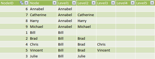
Now, we can use the various Level columns to browse the PivotTable and… well the result is not very sexy. Please note that I removed the city of the invoice from the following reports, to make it simpler to look at the PivotTables.

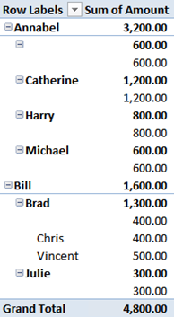
Even if the values are correct, and this time they take into account the hierarchy, there are a few issues:

• Annabel has an empty child (the first one), which is the value of Annabel herself. This happens for all the nodes, up to the level selected. In the figure, I used three levels. Moreover, there is no evidence of the fact that the empty nodes are, indeed, the same value as their parent.
• All three levels are shown, even when they are not useful.

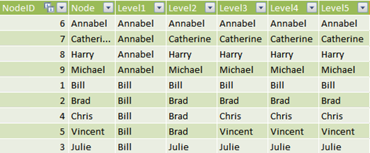
Let us start with solving the first issue. Who are those empty nodes? In the levels, we used NULL for Level2 of Annabel since the node of Annabel has a father at level 1, which is Annabel herself, but no father at levels greater than one. We can assume, with no loss in information, that Annabel is the father of herself for all levels. The same applies for any node: once a node reaches its last level, all the following ones should repeat the node name as its father. Doing so, we will remove all the NULL from the levels, removing empty nodes.

To obtain this result, it is enough to replace the last SELECT of our query with this:

SELECT      NodeId   = C.NodeId,     Node     = T.Node,     Level1   = COALESCE (T1.Node, T.Node),     Level2   = COALESCE (T2.Node, T.Node),     Level3   = COALESCE (T3.Node, T.Node),     Level4   = COALESCE (T4.Node, T.Node),     Level5   = COALESCE (T5.Node, T.Node) FROM      ComputeParentNodeIdAtLevels C         LEFT OUTER JOIN Tree T  ON T.NodeID = C.NodeID         LEFT OUTER JOIN Tree T1 ON T1.NodeID = C.ParentNodeIdAtLevel1         LEFT OUTER JOIN Tree T2 ON T2.NodeID = C.ParentNodeIdAtLevel2         LEFT OUTER JOIN Tree T3 ON T3.NodeID = C.ParentNodeIdAtLevel3         LEFT OUTER JOIN Tree T4 ON T4.NodeID = C.ParentNodeIdAtLevel4         LEFT OUTER JOIN Tree T5 ON T5.NodeID = C.ParentNodeIdAtLevel5

By simply adding the COALESCE, the final table becomes this:

Using this new format for the table, the result is much nicer:

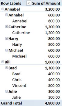
Now all the empty nodes disappeared from the PivotTable, when a node is a leaf it is repeated in all subsequent levels with its name. Still not what we really wanted to show, but definitely better than before.

All what I said up to now, is pretty well known in the BI world. Thus, the interesting part of the post starts here.

Our second goal is to hide all the useless levels. For example, the two “Annabel” under the first one, should be hidden, since Annabel is a level 1 node and should disappear from the PivotTable when Level 2 is browsed. Said in other words, all nodes of level of N-1 should not be made visible at the level N of the hierarchy.

Now, let us try to understand first why the two undesired rows appear in the PivotTable. If we look at the filter contexts of the first three cells of the PivotTable, we get this:

The filter context changes for the three cells. The first cell computes 4 rows, the second and the third ones compute only one row, which is the Annabel row. It is clear that we cannot leverage the fact that there is only one row in the filter context to hide the row because, doing so, we will compute incorrect results for all the leaves. The number of rows in the filter context is note the way to go.

Let us focus on the only row with of Annabel, with NodeID equal to six. It should be computed in the first level and hidden in the next ones. Thus, the DAX formulas will work on the very same row, but with different filter contexts. The key to solve this scenario seems to be to find a way to detect the current filter context and then, if the row should be hidden under the current filter context, find a way to hide it. Unfortunately, in PowerPivot there is no way to compute the current filter context. We can leverage the VALUES function, which will return the distinct values of a column in the current filter context but, in this specific scenario, VALUES (Tree[Filter1]) will return “Annabel” for all the three Filter columns in all of our three contexts. Said in other words, inside DAX there is no way to discriminate computation based on the filter context, we can only discriminate based on the column values and, in our scenario, the column values are always the same.

If we want to be able to discriminate the behavior of DAX in these three filter contexts, we need some column that has a different value in the different filter context. But, in order to do that, we need to have more than one row with the same set of attributes filtered by the contexts and with a new column that has different values in the various filter contexts.

Think in this way: one row contains Annabel and a column which says: “show me in level 1”, another row contains Annabel too but the column will say: “show me in level 2” and so on. This change in the data model will let us discriminate among the various instances of Annabel and let us decide whether a row should be made visible at each level. With this basic idea in mind, we can move a step further and note that we don’t need all of the filter contexts to be different, since we only need to discriminate between levels in which Annabel should be visible and levels in which Annabel should be hidden. Thus, two rows for Annabel are enough, we don’t need a row for each level.

We are moving toward the final solution but, before showing it, it is worth explaining the technique in more detail. If we duplicate the row of Annabel, making some mix between the last two queries (the one with COALESCE and the one without it), we will get this:

Now, these two rows are identical but the first filter context shows both of them, while the second and the third, filtering Level2=”Annabel”, will hide the first row. Now, inside DAX, by counting the rows, we will be able to discriminate between the two situations and we will be able to hide the second instance of Annabel if the first row is not visible. Well, we still need a way to hide the row, but we will come to that later.

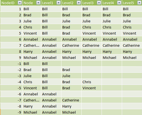
There is still a small problem we have to face before duplicating rows: NodeID is a key in the table and it cannot contain duplicates. Moreover, in the first filter context we want to count Annabel only once, even if there are two rows visible. This is easily accomplished by setting the NodeID of the duplicated row set to a negative value, which is not conflicting with any other ID and does not relate to any row in the fact table.

Since it is clear that the duplication need to affect all the rows (each single row can be visible at a level and hidden at another one), the last SELECT of our query should become:

SELECT      NodeId = C.NodeId,     Node   = T.Node,     Level1 = COALESCE (T1.Node, T.Node),     Level2 = COALESCE (T2.Node, T.Node),     Level3 = COALESCE (T3.Node, T.Node),     Level4 = COALESCE (T4.Node, T.Node),     Level5 = COALESCE (T5.Node, T.Node) FROM      ComputeParentNodeIdAtLevels C         LEFT OUTER JOIN Tree T  ON T.NodeID = C.NodeID         LEFT OUTER JOIN Tree T1 ON T1.NodeID = C.ParentNodeIdAtLevel1         LEFT OUTER JOIN Tree T2 ON T2.NodeID = C.ParentNodeIdAtLevel2         LEFT OUTER JOIN Tree T3 ON T3.NodeID = C.ParentNodeIdAtLevel3         LEFT OUTER JOIN Tree T4 ON T4.NodeID = C.ParentNodeIdAtLevel4         LEFT OUTER JOIN Tree T5 ON T5.NodeID = C.ParentNodeIdAtLevel5 UNION ALL SELECT      NodeID = -C.NodeId,     Node   = T.Node,     Level1 = T1.Node,     Level2 = T2.Node,     Level3 = T3.Node,     Level4 = T4.Node,     Level5 = T5.Node FROM      ComputeParentNodeIdAtLevels C         LEFT OUTER JOIN Tree T  ON T.NodeID = C.NodeID         LEFT OUTER JOIN Tree T1 ON T1.NodeID = C.ParentNodeIdAtLevel1         LEFT OUTER JOIN Tree T2 ON T2.NodeID = C.ParentNodeIdAtLevel2         LEFT OUTER JOIN Tree T3 ON T3.NodeID = C.ParentNodeIdAtLevel3         LEFT OUTER JOIN Tree T4 ON T4.NodeID = C.ParentNodeIdAtLevel4         LEFT OUTER JOIN Tree T5 ON T5.NodeID = C.ParentNodeIdAtLevel5

You can see that I added a UNION ALL and the new rows will contain NULL at the level at which the row should be hidden and the negated ID avoid duplicates and false relationships. The final result looks like this:

Now the data model is ready to be queried, time to move to the PivotTable and take a look at the last points to solve:

• Detect when a row should be hidden
• Find a way to hide it

Let’s go back to our PivotTable, add a measure called CountOfNodeID with the simple formula COUNTROWS (VALUES (Tree[NodeId])), we get this result:

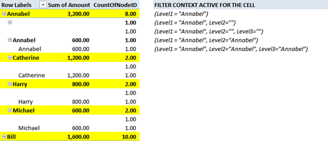
I have highlighted the cells that need to be made visible, all other ones should be hidden. Moreover, this figure makes evident the different filter contexts (now Annabel appears under five different filter contexts, one for the root and two for each level each, where the level is Annabel of NULL). The other thing to note is that all the rows that need to be hidden have a COUNTROWS of 1. This is due to the fact that there are always at least two rows in the filter context, until we reach the point where the NULL value in the level is a discriminant. Then, the two rows are separated into two different contexts, each one of which shows only one of the two rows.

Well, the technique is now clear: we just need to hide all the rows that have a CountOfNodeID that equals to 1. Oh… yes, we still need a way to hide the rows. Ok, last point.

If we remove the CountOfNodeID from the PivotTable, we will get this:

See what happened? All the rows that do not contain a value for Amount disappeared. This is due to the automatic NONEMPTY: all rows with empty values are automatically removed from the final result. Thus, if we put BLANK in a measure, whenever we want to hide a row, that row will automatically disappear from the PivotTable. Let us create a measure, called SumOfAmount, with this formula:

=IF([CountOfNodeID] > 1, SUM (Invoices[Amount]), BLANK ())

Adding it to the PivotTable results in this:

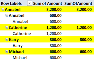
You see that only highlighted rows contain a value for the SumOfAmount measure. Thus, leaving the SumOfAmount measure alone in the PivotTable, we will reach the final result:

Et voilà, the visualization of Parent/Child looks exactly as it looks in SSAS, with no useless nodes. Since the value is computed with a measure, it can be easily sliced using the city of the invoice, as I did in the first figures of this post.

Before going to the end of the post, there are still some small considerations that I want to share.

First. If you want to make it evident the contribution of each node to its total (i.e. Brad has a value of 400 which is not shown in the report, it need to be deduced by the difference between Chris+Vincent and the total of Brad) you can easily add one visible level to the hierarchy, so that each node starts to be hidden one level later. This can be easily accomplished adding a COALESCE to the second part of the query. Another interesting technique is to differentiate between nodes that behave as aggregators and nodes that contain values. In our case, we will end up with two Brad: one who has invoices and another one who is the aggregator. This latter technique, IMHO, leads to a better data model and user experience.

Second. The speed of Parent/Child with this technique is great. In SSAS Parent/Child suffered from the lack of aggregations but, since Vertipaq is superfast without any aggregation, it is still superfast with this implementation of Parent/Child, that behave exactly as any other hierarchy. Try it with your data and share the results, I have not performed many tests on performance and I am eager to see some value published by my readers.

Third. If you need to get the aggregated value in a measure without having the hierarchy displayed on a PivotTable, all of the Level column are of no help. To accomplish that, you need to push the NodePath column computed by the first CTE to the final hierarchy, like this:

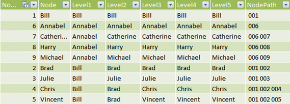
And then, to compute the aggregated value of a node, simply sum up all the rows that contain the NodeID somewhere in the path, using the DAX FIND function which works fine for this. Having used a space as a separator, we will not incur in wrong substring detection. A measure computed in this way can then be used to perform further computation, even if the hierarchy is not visible in the PivotTable.

Fourth: the count of nodes, that determines the visibility of a node, is carried on on the dimension table only. Thus, it runs very fast because there is no need to access the fact table to determine whether a node should be made visible or not. This means that the addition of negative ID in the hierarchy does not affect performances, since those nodes will never be computed against the fact table. Moreover, we need to duplicate the dimension table but this is not very worrying since, normally, dimensions tend to be pretty small (i.e. less than one million rows).

This is a long post so I think a small recap might be useful:

• Since a hierarchy cannot be handled by PowerPivot we need to flatten it using a fixed number of levels. I think ten levels would suffice most scenarios.
• The flattening of the hierarchy need to be done with SQL, since it handles recursion in a snap, while PowerPivot is unable to do this.
• To be able to detect nodes to be hidden, we had to duplicate all nodes in the hierarchy using the Level as the discriminator.
• To hide a row, it is enough to blank ALL the measures shown in the PivotTable and the row will disappear.

And, the most important lesson here is: when formulas tend to look too much complicated, a simple change in the data model will often result in a much cleaner solution. You have seen that the DAX formulas used in this post are really plain, the key of the solution is in the data model, not in the formulas.

To go to a conclusion: Parent/Child hierarchies are not present in PowerPivot, nevertheless they can be implemented pretty well, even if with some SQL and DAX acrobatics. The final result is very nice, elegant as the SSAS implementation is. It works fine and it will benefit from the tremendous speed of the Vertipaq engine providing a great user experience. At the end, it might be the case that PowerPivot handles Parent/Child hierarchies better than SSAS does.

This is just another example of what PowerPivot can do for your reporting needs. If you want to touch the real Karma of PowerPivot, don’t miss the opportunity to follow one of the workshops I and Marco Russo are bringing all over Europe in the next few months.

You can find more info on www.powerpivotworkshop.com. Hope to see you  there!