Explaining REDUCED BY in xmSQL batch events

We recently released the second edition of the Optimizing DAX video course. Despite its volume, some details always did not find space in the training material. The REDUCED BY syntax of xmSQL is one of those details.

What follows is one of the internal notes created during the research for the course. I did not edit it much; you will still find notes and reminders for future investigation.

REDUCED BY and CREATE SHALLOR RELATION appear together in an xmSQL batch to implement a join that potentially produces a cartesian product between two tables.
Regular joins in xmSQL use a regular relationship and work on an expanded table.
REDUCED BY enables an INNER JOIN that works on a cartesian product (like in SQL) mapped on a relationship defined in the batch.
The relationship (CREATE SHALLOW RELATION) can be generated by a CROSSFILTER or a TREATAS in DAX (note: not sure whether there could be other cases) and must be defined in the batch to enable the relationship use in an INNER JOIN. We could say that INNER JOIN is always tied to REDUCED BY, which requires a SHALLOW RELATION.

The table that appears after REDUCED BY is the main table of the join, and it usually has aggregations – because, in the absence of aggregation, there is probably no reason for such a cartesian product.
Consider this query:

EVALUATE
SUMMARIZECOLUMNS (
    Customer[Continent],
    "Amt",
        CALCULATE (
            DIVIDE (
                SUMX ( Sales, Sales[Quantity] * Sales[Net Price] ),
                COUNTROWS ( Customer )
            )
        )
)

In SQL we would not have such a constraint; we can write:

SELECT …
FROM ( 
    SELECT Customer.x, COUNT ( Customer.x )
    FROM Customer
    GROUP BY Customer.x
) C
INNER JOIN (
    SELECT Sales.x, SUM ( Sales.y )
    FROM Sales
    GROUP BY Sales.x
) S
ON S.x = C.x

In xmSQL, a direct join can be created only when a regular relationship exists.

Let us remove the relationship and use TREATAS to move the filter. We no longer join across the expanded table, so LEFT OUTER JOIN is no longer an option, and INNER JOIN must be used, potentially with a Cartesian product that could inflate values – even though xmSQL does not know that.

EVALUATE
SUMMARIZECOLUMNS (
    Customer[Continent],
    "Amt",
        CALCULATE (
            DIVIDE (
                SUMX ( Sales, Sales[Quantity] * Sales[Net Price] ),
                COUNTROWS ( Customer )
            ),
            CROSSFILTER ( Sales[CustomerKey], Customer[CustomerKey], NONE ),
            TREATAS ( VALUES ( Customer[CustomerKey] ), Sales[CustomerKey] )
        )
)

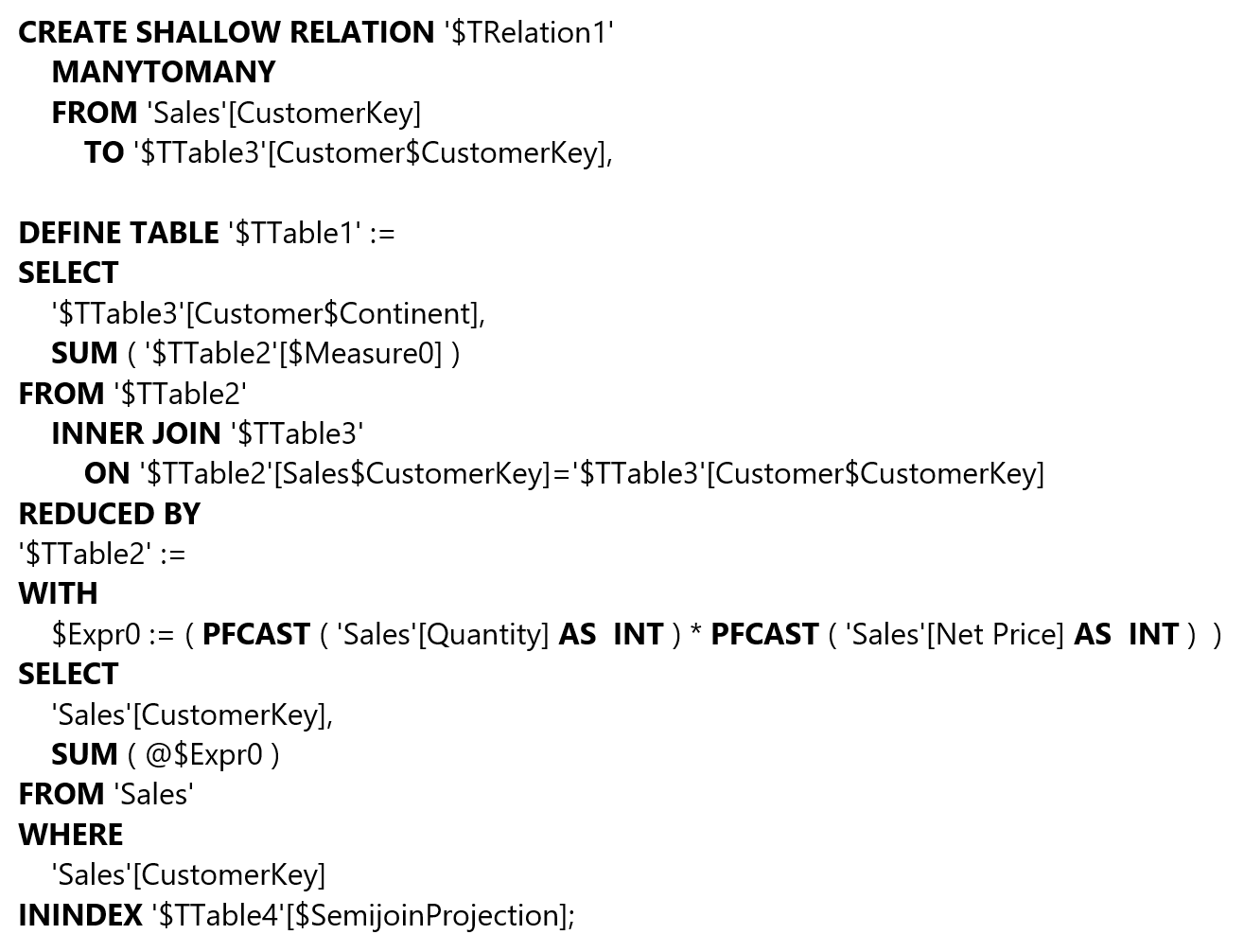
The presence of INNER JOIN requires a table specified by REDUCED BY:

The query after REDUCED BY, in reality, is the “main” query that will be grouped by conditions defined in the query before “REDUCED BY”.
The query before REDUCED BY usually has grouping columns and potentially a smaller table (in this case, the Customer dimension).
We can see REDUCED BY as a way to join two subqueries using a relationship (with INNER JOIN) that is not defined in the model.
REDUCED BY cannot use LEFT OUTER JOIN and cannot produce blank rows (this also relates to the behavior of the “blank row” in DAX).
In the previous example, we forced the engine to use REDUCED BY, because we removed the regular relationship from the available metadata.

The engine does not know that the result can be aggregated. Another way to see this is that with a LEFT OUTER JOIN, every row of the table on the left side is grouped only in one group produced in the output.
When we have an INNER JOIN with REDUCED BY, every row in the table after REDUCED BY can be grouped in multiple rows of the result. The measure is non-additive in that case, and we can assume that the cost is higher than a regular relationship by orders of magnitude (note: I would have guessed that a scan of the “reduced by” table is required for each group of the result, whereas with a LEFT OUTER JOIN a single scan of the table on the many-side was required – however, performances do not back this theory, it seems that the main variables are the size of the two joined tables, with the output number of rows playing a minor role; probably more investigation is required).

The INNER JOIN / REDUCED BY is needed to join a table with virtual relationships. A bidirectional filter works like a virtual relationship; the only difference is the time required to build the table used in the batch to complete the join (note: this is out of scope by now, but we could investigate deeper on this difference).
Consider this non-additive DAX query:

EVALUATE
SUMMARIZECOLUMNS (
    Customer[Continent],
    "Amt",
        CALCULATE (
            DIVIDE (
                SUMX ( Sales, Sales[Quantity] * Sales[Net Price] ),
                COUNTROWS ( 'Product' )
            ),
            CROSSFILTER ( Sales[ProductKey], 'Product'[ProductKey], BOTH )
        )
)

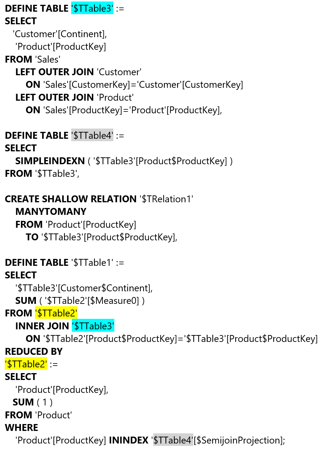
The complete xmSQL code has the same structure as the previous one where we used TREATAS – the following xmSQL query only solves the COUNTROWS ( Product ) part of the DAX query, and the Sales Amount is computed in another xmSQL query (focus on $TTable2 and $TTable3 that are used in the INNER JOIN and REDUCED BY syntax):

Thus, an xmSQL query can aggregate non-additive measures using INNER JOIN + REDUCED BY.

Let us see the difference between a regular relationship with a bidirectional filter and a virtual relationship obtained using TREATAS. Consider this variation of the previous DAX query:

EVALUATE
SUMMARIZECOLUMNS (
    Customer[Continent],
    "Amt",
        CALCULATE (
            DIVIDE (
                SUMX ( Sales, Sales[Quantity] * Sales[Net Price] ),
                COUNTROWS ( 'Product' )
            ),
            TREATAS ( VALUES ( Sales[ProductKey] ), 'Product'[ProductKey] )
        )
)

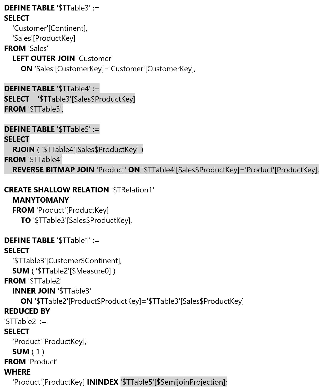
This is the xmSQL code – the only difference is the table used to filter the semijoin projection:

The use of RJOIN is probably related to the usual conditions (the 1:M ratio of the relationship), and performance may differ depending on the conditions. There are certainly cases where the TREATAS approach results in being faster and others where it is slower. (note: we probably should investigate more on that to provide better guidance – however, it seems that this could be relevant only when the cost of creating this relationship is significative compared to the cost of the aggregation used later; otherwise, it could be not noticeable as the remaining part of the xmSQL batch is identical).