Computing open orders with visual calculations in DAX

Open orders (or events in progress) is an extremely common pattern in business intelligence. It answers a simple question: given two dates – order received and order delivered – how many orders have yet to be delivered at any given point? We do have a pattern here: Events in progress – DAX Patterns that solves the scenario with DAX measures.

While demonstrating the pattern during a classroom course, one student (thanks Justin Duff!) asked whether the pattern could be solved by using visual calculations. It turns out that visual calculations can be of great help in optimizing the performance of this specific scenario because they greatly reduce the number of calculations required to solve it. Well… sort of. Visual calculations might perform well, but we will do better with DAX alone!

In this article, we first outline one possible solution for open orders. That solution is not the most optimal in general. However, outlining the algorithm is useful from an educational standpoint. We then quickly analyze the performance of that solution, and finally we rewrite the solution by using visual calculations. To do this, we take advantage of the fact that visual calculations compute running totals on top of the virtual table rather than relying on the data model only. This simple fact greatly helps in reducing the complexity of the calculation. Finally, we show that the greatest strength of visual calculations is also their worst problem: data outside of the virtual table cannot be accessed. However, by mixing visual calculations and some DAX measures we obtain a nice and efficient solution.

As is always the case in technology, different tools are not to be considered as rivals; instead, the wise developer uses different tools together as a powerful team to achieve the best solutions. Before we conclude the article, we use everything we found out with visual calculations to obtain even better performance with a regular DAX measure only. In doing so, we obtain the best of both worlds: an optimized measure that works in the model and runs even faster than visual calculations do. The takeaway of the article is thus that you can solve the same scenario in multiple ways: the more tools you know, the more ideas you can explore to find the best possible option.

Computing with simple DAX measures

For this demo, we focus on two tables only: Sales and Date. They have two relationships between them, one with Order Date and the other with Delivery Date.

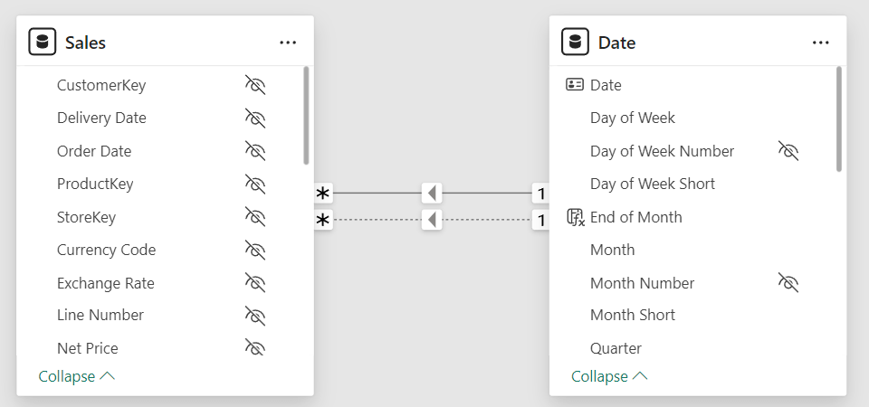
Based on this model, two simple measures compute the number of orders received and delivered:

Orders Received = DISTINCTCOUNT ( Sales[Order Number] )

Orders Delivered =
CALCULATE (
    [Orders Received],
    USERELATIONSHIP ( Sales[Delivery Date], 'Date'[Date] )
)

Before moving forward, please note that the Orders Received base measure computes a distinct count. Distinct counts have two unfortunate properties: they may be slow, and they cannot be aggregated as an additive measure. These two issues will produce serious performance challenges in the next calculations.

Let us start by looking at the result we want to obtain: a report showing, for each month, the number of orders received, the number of orders delivered, and the number of orders still open at the end of the period.

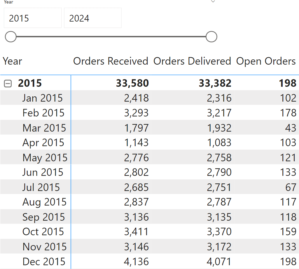
Look at Feb 2015: there were 102 orders open in January; 3,293 orders were received; 3,217 orders were delivered; there are 178 remaining orders. The math is very simple: the previous value of open orders, plus the orders received, minus the orders delivered. However, expressing the same calculation in DAX requires some effort because there is no easy way to retrieve the value of a column in the previous row.

One possible solution is to create a measure that computes the running total of both the orders received and the orders delivered. With such measures, computing the open orders becomes a simple subtraction:

Received RT =
CALCULATE (
    [Orders Received],
    'Date'[Date] <= MAX ( 'Date'[Date] )
)

Delivered RT =
CALCULATE (
    [Orders Delivered],
    'Date'[Date] <= MAX ( 'Date'[Date] )
)

OpenOrders =
[Received RT] - [Delivered RT]

The next figure shows the values of the two running totals. You can verify that the number of open orders is indeed a simple subtraction of the two measures.

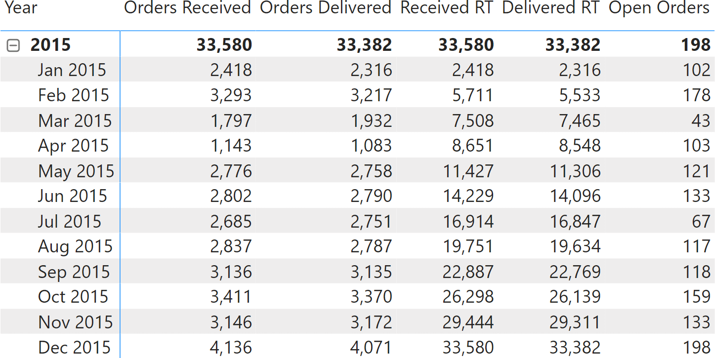
These measures compute the correct value. The problem is performance. Both running totals require a scan of the entire Sales table to compute a distinct count. Because distinct counts cannot be aggregated, each cell must be computed separately. The sample data model contains 10 years of data, corresponding to 112 months (the last year is not complete). Therefore, we expect the query that computes the report to run more than 112 queries, each of which requires a scan of the entire Sales table. Moreover, each cell requires computing both the orders received and delivered. Because the two measures use two different relationships, two queries are needed for each. In other words, a rough count states that more than 224 queries are needed, not counting subtotals and other smaller queries.

Indeed, executing the query to compute only Open Orders produces the following result.

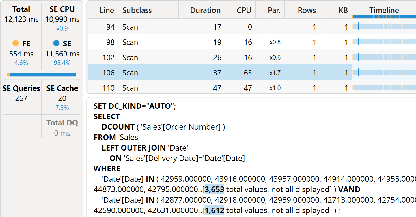
The whole query runs in more than 12 seconds. There are 267 queries, as expected, most of which are in the form of the one highlighted: a distinct count over Sales with a filter over Date. The filter includes a large set of dates. Each query is pretty fast, but there are so many that the query ends up performing poorly. The more rows shown in the report, the slower the query will be.

The main issue with this calculation is that when the engine computes the value for February, it cannot rely on the value already computed for January. This type of incremental calculation is extremely simple to obtain in other tools like Excel, whereas it is very complex with DAX. True, the window functions are designed to simplify scenarios like this one. However, window functions are not of great help here because the calculation requires a distinct count; therefore, it is not additive.

The following measure computes open orders with a window function, and still performs rather slowly:

Open Orders Window = 
CALCULATE (
    CALCULATE ( 
        [Orders Received] - [Orders Delivered],
        WINDOW ( 0, ABS, 0, REL, ALL ( 'Date'[Date] ) )
    ), 
    'Date'[Date] = MAX ( 'Date'[Date] )
)

Computing with visual calculations

In this scenario, visual calculations are of great help. Using a visual calculation, we can build a report that computes the two base calculations (Orders Received and Orders Delivered). Then, the running total would be computed on top of these precomputed values, thus avoiding having to scan the Sales table again. The virtual table contains one row per month, which strongly reduces the computational effort.

Starting from a matrix that contains Orders Received and Orders Delivered, we can compute three visual calculations:

Received RT = RUNNINGSUM ( [Orders Received], ROWS )

Delivered RT = RUNNINGSUM ( [Orders Delivered], ROWS )

Open Orders = [Received RT] - [Delivered RT]

RUNNINGSUM is nothing magical: it still uses a window function. What really changes is the granularity of the table being used: rather than Sales, the engine now uses the virtual table. The gain in terms of performance is tremendous.

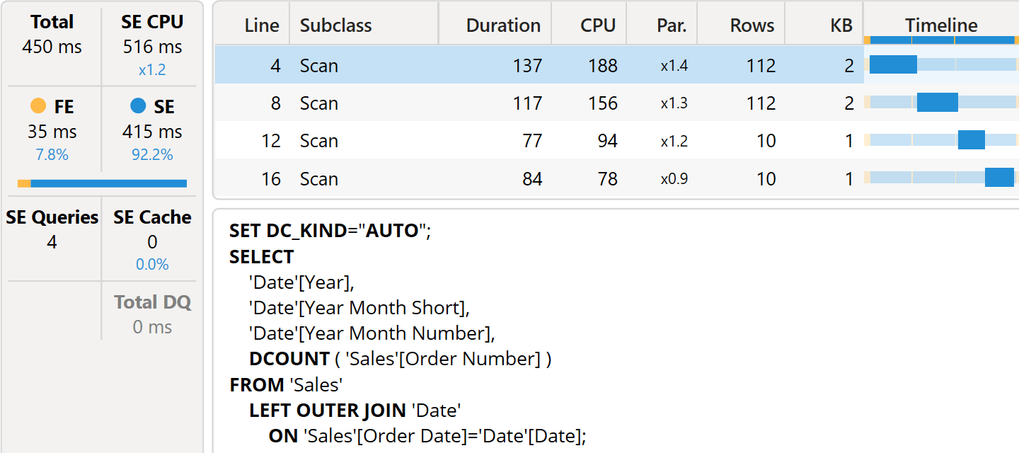
Using visual calculations, there are now only four queries to compute both the raw values and the subtotals. Visual calculations compute their results based on the data already pre-aggregated, and this simple fact produces incredibly good results in this type of scenario.

However, this very same fact proves to be an issue. If a user adds a slicer by year, visual calculations will provide the calculation starting from the first of the selected years, as if it were the first year in the model. Hence, the result would be wrong.

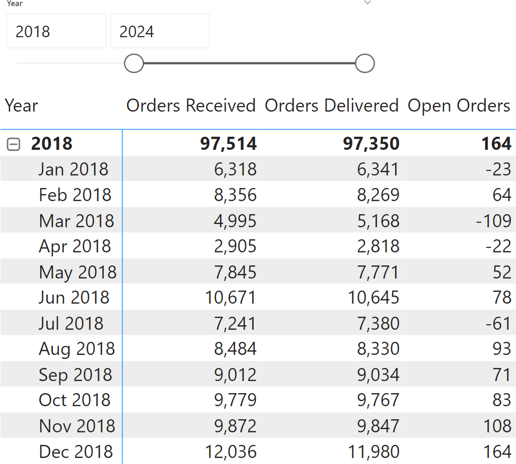
The result for Jan 2018 cannot be a negative number. While it is true that more orders were delivered than received, the calculation does not consider the backorder left in December 2017. The thing is: the virtual table does not contain any information about what happened before 2018. Moreover, a visual calculation cannot access the data model to inspect data not already present in the virtual table.

The solution is to create a model measure that computes the starting value for the open orders, that is, the value left before the beginning of the current visual – in our example, the value left at the end of 2017:

Starting Value for Open Orders = 
CALCULATE (
    VAR FirstDateInVisual = MIN ( 'Date'[Date] )
    RETURN 
    CALCULATE (
        [Received RT] - [Delivered RT],
        'Date'[Date] < FirstDateInVisual
    ),
    ALLSELECTED ( 'Date' )
)

This calculation produces the same number for all the rows, because of ALLSELECTED. We use the value in the computation of Open Orders:

Open Orders = [Starting Value for Open Orders] + [Received RT] - [Delivered RT]

There is a small price to pay in terms of performance because of the additional column, but this modification makes the visual calculation version work.

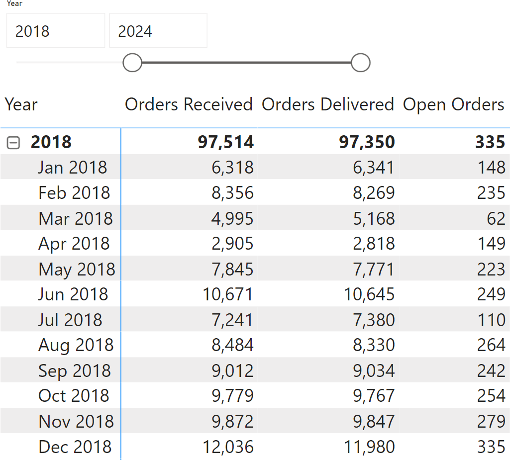
As you have seen, visual calculations are extremely useful in this scenario, because they strongly reduce the complexity of the measure. However, visual calculations alone would not be able to solve the scenario. With a little help from a DAX regular measure, the problem can be solved efficiently.

Optimizing DAX measures

Now that we have a better understanding of a good algorithm to compute the open orders calculation, we can write a DAX version that uses the same technique. We create a temporary table with the orders received and the orders delivered, and then we iterate over the temporary table to compute each cell rather than scanning Sales every time:

Open Orders DAX Opt = 
VAR Deltas = 
    ADDCOLUMNS (
        ALL ( 'Date'[Date] ),
        "@Delta", [Orders Received] - [Orders Delivered]
    )
VAR MaxDate = MAX ( 'Date'[Date] )
VAR Result = 
    SUMX ( 
        FILTER ( Deltas, 'Date'[Date] <= MaxDate ),
        [@Delta]
    )
RETURN
    Result

It is worth noting that this DAX version computes the table in the Deltas variable at the day granularity, rather than at the month granularity as the virtual table in the visual calculation version does. This is not strictly needed, but it is good to have so the measure works at any granularity. We could have created a slightly faster version using the Month Number column to reduce the computational complexity further, but it would have been less flexible.

The thing is, with this non-super-duper-optimal version, the measure is already running faster than the visual calculation.

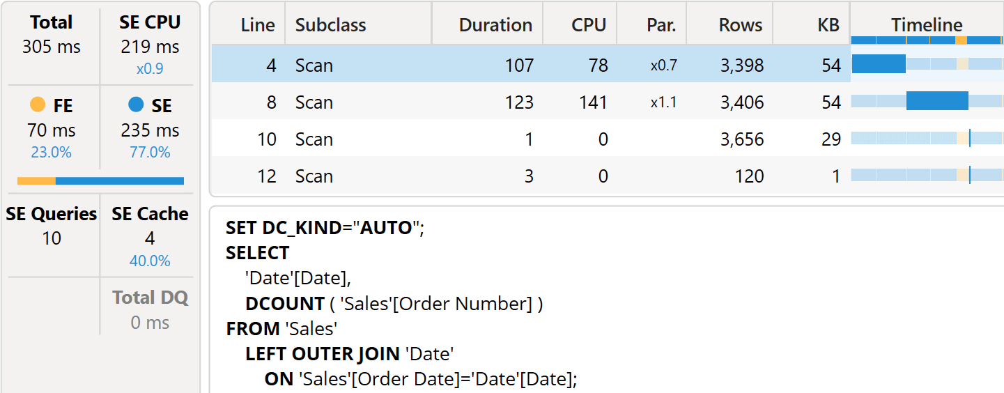
As you see, the storage engine query retrieves the orders received at the date granularity, making the measure very versatile.

Conclusions

In this scenario, the main advantage of visual calculations is their simplicity. The calculation is simple to author and much faster than a naïve version written in regular DAX. However, writing optimized DAX proves to be even faster than a visual calculation. Moreover, the visual calculation version still requires some DAX knowledge to obtain the opening balance of the open order calculation.

Needless to say, this does not mean that – as a rule – visual calculations are slower than regular DAX, or that they are always faster. Each scenario is unique and requires a deep study by a DAX professional to implement the optimal solution.

However, visual calculations can provide good performance in some scenarios to any users, regardless of their DAX competencies. In our case, they proved to be a useful tool to test some techniques that can be later expressed with regular DAX and better performance.